STAD70

Statistics & Finance II §

Taught by Sotirios Damouras.
PDF version here

W1: Financial Data & Returns §

Continuous double auction §

• Real-time mechanism to match buyers & sellers and determine prices at which trades execute
• At any time, participants can place orders in the form of bids (buy) and asks (sell)
• Matching orders (bid $\ge$ ask) are executed right away, whereas outstanding orders are maintained in an order book

Order types §

• Limit order: transact at no more/less than a specific price
  • If order not filled, it’s kept in the order book
• Market order: transact immediately at current market price
  • A single order can have more than one price
• Iceberg order: contains both hidden and displayed liquidity
  • Splits a large order into smaller ones to maintain order anonymity

Financial data §

• Quote data: record of bid/ask prices from order book
• Trade data: record of filled orders

Daily data §

• Open/close
  • Adjusted close (used for calculating returns): adjusted for dividends and splits
• High/low
• Volume

Candlestick §

• Green: close > open
• Red: close < open

Other data §

• FX rates: currency prices set by global financial centers
• LIBOR rates: average interest rate that major London banks would be charged when borrowing from each other

Reliability of financial data §

Financial data could be skewed by

• Fake orders: trades placed to manipulate prices w/o intention to trade
• Fake trades: trades where buyer and seller is the same party, used to increase trading activity

Returns §

$R_t=\frac{P_t-P_{t-1}}{P_{t-1}}=\frac{P_t}{P_{t-1}}-1$

Log returns (assumes continuous compounding) §

$$r_t=\log \left(1+R_t\right)=\log \left(\frac{P_t}{P_{t-1}}\right)=\underset{p_t}{\underbrace{\log \left(P_t\right)}}-\log \left(P_{t-1}\right)=p_t-p_{t-1}$$

Dividend adjustment §

Assuming dividend is reinvested, the adjusted return is

$$\begin{array}{rl}& R_t=\frac{P_t+D_t}{P_{t-1}}-1\\ & r_t=\log \left(P_t+D_t\right)-\log \left(P_{t-1}\right)\end{array}$$

The dividend is added back to the price (after the price drop)

Split adjustment §

$$\begin{array}{rl}& R_t=\frac{P_t}{P_{t-1}/2}-1\\ & r_t=\log \left(P_t\right)-\log \left(P_{t-1}/2\right)\end{array}$$

Net vs log returns §

$R_t\approx r_t$ for small values of $R_t$ (<1%)

Taylor approx.: $f(x)\approx f(x_0)+f^{\prime }(x_0)(x-x_0)+\frac{1}{2}{f}^{\prime \prime }(x_0)(x-x_0{)}^2+...$

$$\begin{array}{rl}{r}_t& =\log (\underset{x}{\underbrace{1+R_t}})\leftarrow \text{ expand log function around }{x}_0=1\\ r_t& \approx \log (1)+{\log }^{\prime }(x){|}_{x=1}\cdot (\underset{x}{\underbrace{1+R_t}}-\underset{x_0}{\underbrace{1}})+...\\ & =0+\frac{1}{1}{R}_t\\ & \approx R_t\end{array}$$

Monthly returns §

For daily net returns $R_1,R_2,\dots ,R_{22}$, monthly net return is:

$$R_{1-22}=\left(1+R_1\right)\times \left(1+R_2\right)\times \cdots \times \left(1+R_{22}\right)-1$$

For daily log returns $r_1,r_2,\dots ,r_{22}$, monthly log return is:

$$\begin{array}{rl}{r}_{1-22}& =\log (\frac{P_{22}}{P_{21}}\frac{P_{21}}{P_{20}}...\frac{P_1}{P_0})\\ & =\log (\frac{P_{22}}{P_{21}})+\log (\frac{P_{21}}{P_{20}})+...+\log (\frac{P_1}{P_0})\\ & =r_1+r_2+\cdots +r_{22}\end{array}$$

Random walk model §

Additive log returns suggest using the following to model asset prices

$$\log (\frac{P_t}{P_0})=r_1+r_2+...+r_t$$

If $\{r_t\}$ are i.i.d., then the log return process is a RW with drift $\mu$ and volatility $\sigma$

• aggregate returns over $n$ periods has mean $n\mu$ and volatility $\sqrt{n}\sigma$

Exponential/geometric random walk §

$$P_t=P_0\exp \{r_1+...+r_t\}$$

Return distribution §

• Most convenient assumption: normal (by CLT)
  • Not a good description of reality due to fat tails (heavier than normal)
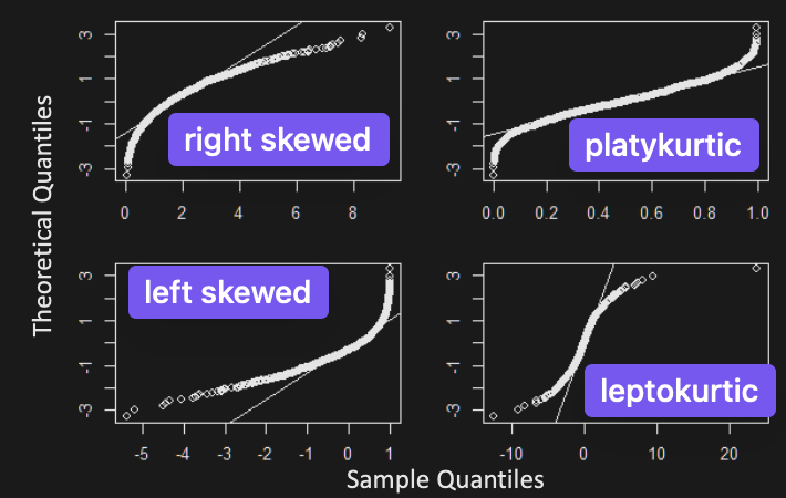
• Skewness = $E\left[{\left(\frac{X-\mu }{\sigma }\right)}^3\right]$
  • Right skewed $⟺$ positively skewed
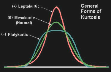
• Kurtosis = $E\left[{\left(\frac{X-\mu }{\sigma }\right)}^4\right]-3$

  • Measures heaviness of the tails

  • Defined as the standardized fourth central moment of a distribution minus 3, which is the kurtosis of the standard normal distribution

  • Returns are leptokurtic

    

E.g. Identify skewness/kurtosis from QQ plot §

W2: Univariate Return Modelling §

Normality tests §

• Kolmogorov-Smirnov - Based on distance of empirical & Normal CDF
• Jarque-Bera - Based on skewness & kurtosis combined
• Shapiro-Wilk (most powerful) - Based on sample & theoretical quantiles (QQ plot)

Heavy tail distributions §

A pdf $f(x)$ is said to have:

• Exponential tails, if $f(x)\propto \exp (-x/\lambda )$
• Polynomial tails, if $f(x)\propto x^{-(1+\alpha )}$

Heavy tailed distributions are those with polynomial tails.

• $\alpha$ is the tail index controlling tail weight: smaller $⟺$ heavier tails
• for $k\ge \alpha$, moments are infinite: $E(X^k)=\infty$
  • Although the MGF’s is infinite, the characteristic function always exists (refer to PS2 Q2)

Examples §

Pareto

$$f(x)=\frac{\alpha x^{-\alpha +1}}{l^{\alpha }}$$

Cauchy: $\alpha =1$

$$f(x)=\frac{1}{\pi (1+x^2)}$$

Student’s t: $\alpha =\nu$

$$f(x)=\frac{\Gamma (\frac{\nu +1}{2})}{\sqrt{\nu \pi }\Gamma (\frac{\nu }{2})}(1+\frac{x^2}{\nu }{)}^{-\frac{\nu +1}{2}}$$

Theoretical justification §

Let $r_1,\dots ,r_n\sim$ i.i.d. heavy tail distributions with tail index $0<\alpha <2$

By the generalized CLT, the aggregate return $r_{1\to n}=r_1+\dots +r_n\sim$ stable distribution

A distribution is stable if linear combinations of independent RVs have the same distribution, up to location and scale parameters.

• All stable distributions besides the Normal have heavy tails, but not all heavy tailed distributions are stable (unstable if tail index > 2)
• Moreover, the sum of independent stable RVs also follows a stable distribution
• Thus, adding many heavy tail $(\sigma =\infty )$ i.i.d. price changes, we get heavy tail returns

Modeling tail behaviour §

The complementary CDF of a heavy tail distribution behaves as:

$$\bar{F}(x)=1-F(x)=P(X>x)\sim x^{-\alpha }\text{, as }x\uparrow$$

To model (absolute) returns above a cutoff $r_{\text{min }}$, use Pareto distribution $\bar{F}(r)={\left(r/r_{\min }\right)}^{\alpha },\forall r>r_{\min }$

To estimate tail index $\alpha$, use:

• Maximum Likelihood: $\hat{\alpha }=\frac{n}{{\sum }_{i=1}^n\ln \left(r_i/r_{\min }\right)}$
• Pareto QQ plots (for tails, e.g. top 25% of returns):
  • Plot empirical CDF vs returns in log-log-scale
  • Estimate $\alpha$ using slope of best fitting line (simple linear regression)
• Student’s t QQ plot (for entire distribution, not just tails)
  • Adjust for location and scale $Y=\mu +\sigma X$ where $X\sim t(\nu ),\{\begin{array}{l}E(X)=0\\ V(X)=\frac{\nu }{\nu -2}\end{array}$
  • Estimate parameters $(\mu ,\sigma ,\nu )$ using MLE
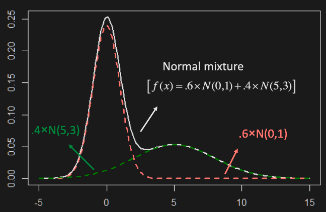
• Mixture models
  • Generate an RV from one out of a family of distributions, chosen at random according to another distribution (a.k.a. mixing distribution)
    • Easy to generate, but not easy to work with analytically
  • 2 types: discrete and continuous
    • e.g. (discrete mixing distribution) RV generated from $\{\begin{array}{ll}N(0,1)& p=60\%\\ N(5,3)& p=40\%\end{array}$
      • 
  • e.g. (continuous mixing distribution) $Y=\mu +\sqrt{V}\cdot Z$ where $V$ is a RV. This is called a normal scale mixture.
    • Examples with heavy tails:
      • (GARCH) $r_t=\mu +{\sigma }_t{Z}_t$ where the mixing process for ${\sigma }_t$ is ${\sigma }_t^2=\omega +{\sum }_{i=1}^p{\alpha }_i{r}_{t-i}^2+{\sum }_{j=1}^q{\beta }_j{\sigma }_{t-j}^2$
      • (T-dist) $t=Z\sqrt{\nu /W}$ where $W\sim {\chi }^2(df=\nu )$

E.g. using mixture models, verify that for $X\sim t(\nu )$, $\{\begin{array}{l}E(X)=0\\ V(X)=\frac{\nu }{\nu -2}\end{array}$

Hint: if $W\sim {\chi }^2(\nu )$, then $E(1/W)=1/(\nu -2)$.

$E(t)=E(Z\sqrt{\nu /W})=\underset{0}{\underbrace{E(Z)}}E(\sqrt{\nu /W})=0$

$V(t)=E(t^2)-\underset{0}{\underbrace{[E(t){]}^2}}=E\left(Z^2\cdot \frac{\nu }{W}\right)=E(Z^2)E\left(\frac{\nu }{W}\right)=1\cdot \nu E\left(\frac{1}{W}\right)=\frac{\nu }{\nu -2}$

Stylized Facts §

Typical empirical asset return characteristics:

1. Absence of simple autocorrelations
2. Volatility clustering
3. Heavy tails
4. Intermittency (alternation between periodic and chaotic behaviour)
5. Aggregation changes distribution (the distribution is not the same at different time scales)
6. Gain/loss asymmetry

Extreme value theorem §

2 limit results for modelling extreme events that happen with small probability

1st EVT (Normalized max of an iid sequence converges to the generalized extreme value distribution) §

Let $X_1,X_2,...$ be i.i.d. RVs and $M_n=\max (X_1,...,X_n)$.

$\exists$ normalizing constants $a_n>0,b_n$ s.t.

$$P\left(\frac{M_n-b_n}{a_n}\le x\right)={\left[F\left(a_{n}x+b_n\right)\right]}^n\to H(x)$$

If $H(x)$ exists, it must be one of:

$$\begin{array}{rl}\text{Gumbel (exponential tails): }H(x)& =\exp \left\{-e^{-x}\right\},x\in \mathbb{R}\\ \text{Frechet (heavy tails): }H(x)& =\{\begin{array}{cc}0& x<0\\ \exp \left\{-x^{-\alpha }\right\}& x>0\end{array}\\ \text{Weibull (light/finite tails): }H(x)& =\{\begin{array}{cc}\exp \left\{-|x{|}^{\alpha }\right\}& x<0\\ 1& x>0\end{array}\end{array}$$

We can combine the three types into the generalized extreme value distribution

$$H(x)=\exp \left\{-{\left(1+\xi \frac{x-\mu }{\sigma }\right)}_{+}^{-1/\xi }\right\}$$

$\xi$ is the shape parameter:

• $>0$ for heavy tails
• $=0$ for exponential tails
• $<0$ for light tails

E.g. Show that the “normalized” max of iid Uniform (0, 1) with $a_n=\frac{1}{n}$, $b_n=1$ converges to Weibull for $x<0$

$$\begin{array}{rl}P(\frac{M_n-b_n}{a_n}\le x)& =P(\frac{M_n-1}{1/n}\le x)=P(M_n\le \frac{x}{n}+1)\\ & =P(\max (U_1,...,U_n)\le 1+\frac{x}{n})\\ & =\prod _{i=1}^{n}P(U_i\le 1+\frac{x}{n})\\ & =(1+\frac{x}{n}{)}^n=(1-\frac{|x|}{n}{)}^n\\ \underset{n\to \infty }{\lim }(1-\frac{|x|}{n}{)}^n& =e^{-|x|}\leftarrow \text{ CDF for Weibull with }\alpha =1\end{array}$$

2nd EVT (Conditional distribution converges to GPD above threshold) §

For RV $X$ with CDF $F(\cdot )$, consider its conditional distribution given that it exceeds some threshold $u$:

$$F_u(y)=\frac{F(u+y)-F(u)}{1-F(u)},0\le y\le x_F-u$$

​where $x_F=\sup \{x\in \mathbb{R}:F(x)<1\}$ is the right endpoint (finite or $\infty$) of $F$

In certain cases, as $u\to x_F$, the conditional distribution converges to the same (family of) distributions called the Generalized Pareto Distribution (GPD)

$$\begin{array}{rl}{F}_u(y)\to G_{\xi ,\sigma }(y)& =1-{\left(1+\xi \frac{y}{\sigma }\right)}_{+}^{-1/\xi }\\ & =\{\begin{array}{ll}1-{\left(1+\xi \frac{y}{\sigma }\right)}^{-1/\xi }& \xi \ne 0\\ 1-e^{-y/\sigma },& \xi =0\end{array}\end{array}$$

where $\sigma >0,y\ge 0$, and for $\xi <0,y\le -\sigma /\xi$

This gives:

• $\xi >0$ : heavy tails (tail index $1/\xi$ )
• $\xi =0$ : exponential distribution
• $\xi <0$ : finite upper endpoint

W3: Multivariate Modeling §

We can model the returns of a linear combination of assets using a constant matrix $A$ like so

$$Cov(A^{T}R)=A^{T}Cov(R)A$$

To minimize the effect of outliers, we can use robust estimation - an estimation technique that is insensitive to small departures from the idealized assumptions that were used to optimize the algorithm

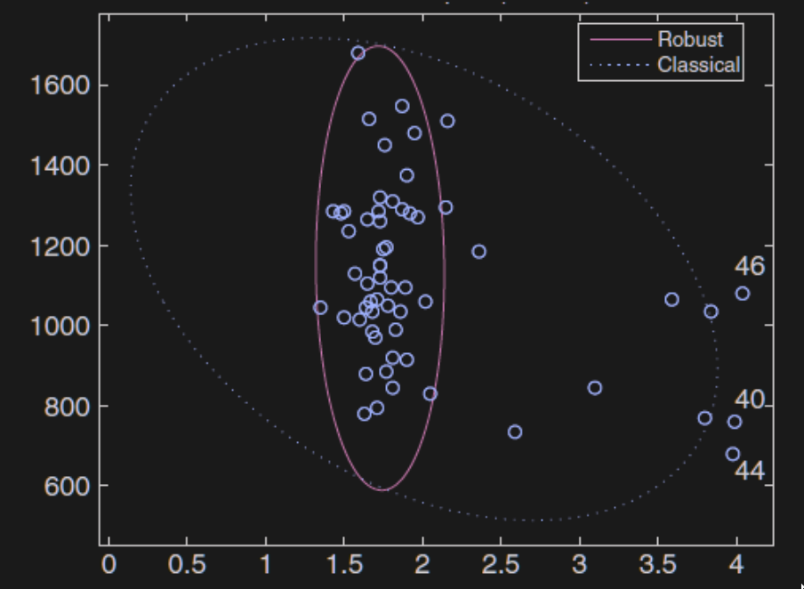
However, we should never remove outliers in finance. We can instead model heavy tails using the following.

Multivariate (Student’s) t distribution §

A more practical/realistic distribution than Normal for modelling financial returns.

$\mathbf{R}=\mathbf{\mu }+\mathbf{Z}\sqrt{\nu /W}$ where $Z\sim N(0,\mathbf{\Lambda }),W\sim {\chi }^2(df=\nu )$

Note that it is a Normal that gets scaled/divided by the square root of a Chi-square

Notation: $\mathbf{R}\sim t_{\nu }(\mathbf{\mu },\mathbf{\Lambda })$ where $\mathbf{\Lambda }=Cov(Z)$, not $Cov(R)$

$E(R)=E(Z)$, but $Cov(Z)\ne Cov(R)$

• $E(R)=E(\mu +Z\sqrt{\nu /W})=\mu +\cancel{E(Z)}\cdot E(\sqrt{\nu /W})=\mu$
• $Cov(R)=Cov(\mu +Z\sqrt{\nu /W})=Cov(Z)Cov(\sqrt{\nu /W})=\Lambda \frac{\nu }{\nu -2}\text{ for v>2}$

Marginals are t-distributed with the same degrees of freedom $⟹$ all asset returns have the same tail index $\alpha$

There is tail dependence - extreme values are observed at the same time in all dimensions (desirable property for modelling financial returns)

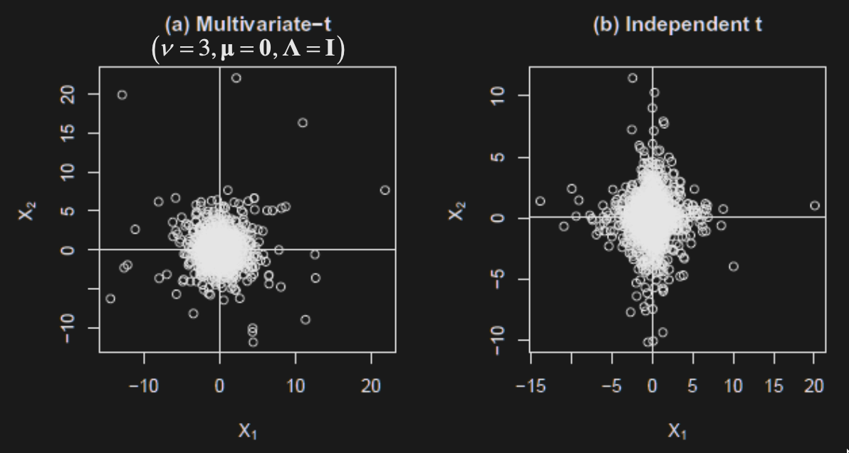
The greater the tail dependence, the more points we will observe in the corners (figure on the left has tail dependence).

Linear combinations of multivariate t follow 1D t with the same df

$\mathbf{R}\sim t_{\nu }(\mathbf{\mu },\mathbf{\Lambda })⟹{\mathbf{w}}^T\mathbf{R}\sim t_{\nu }({\mathbf{w}}^T\mathbf{\mu },{\mathbf{w}}^T\mathbf{\Lambda }\mathbf{w})$

• $E({\mathbf{w}}^{T}R)={\mathbf{w}}^{T}E(R)$
• $Var({\mathbf{w}}^{T}R)={\mathbf{w}}^{T}Var(\mu +Z\sqrt{\frac{\nu }{\mathbf{w}}})\mathbf{w}={\mathbf{w}}^T\underset{\Lambda }{\underbrace{Var(Z)}}Var(\sqrt{\frac{\nu }{\mathbf{w}}})\mathbf{w}=\frac{\nu }{\nu -2}({\mathbf{w}}^T\Lambda \mathbf{w})$

Using the same degree of freedom is limiting. A more flexible way is to model dependencies with copulas.

Copula §

Intuitively, copulas allow us to decompose a joint probability distribution into the following:

• their marginals (which by definition have no correlation)
• a function which couples them together

thus allowing us to specify the correlation separately. The copula is that coupling function. (joint = copula + marginals)

Formally, a copula is a multivariate CDF with Uniform(0, 1) marginals

$C(u_1,...,u_d)\in [0,1],\forall u_1,...,u_d\in [0,1]$

• $C(0,...,0)=0$
• $C(1,...,1)=1$
• $C(...,u_{i-1},0,u_{i+1},...)=0$
• $C(1,...,1,u_i,1,...,1)=u_i$

Independence copula §

$C_{\text{indep }}\left(u_1,\dots ,u_d\right)=u_1\times \cdots \times u_d$

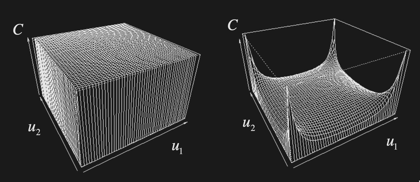
Fréchet-Hoeffding theorem (Copula bounds) §

Any copula is bounded like so

$$\begin{array}{rl}& \underline{C}\left(u_1,\dots ,u_d\right)\le C\left(u_1,\dots ,u_d\right)\le \bar{C}\left(u_1,\dots ,u_d\right)\\ & \text{ where }\{\begin{array}{l}\underline{C}\left(u_1,\dots ,u_d\right)=\max \left\{0,1-d+{\sum }_{i=1}^d{u}_i\right\}\\ \bar{C}\left(u_1,\dots ,u_d\right)=\min \left\{u_1,\dots ,u_d\right\}\end{array}\end{array}$$

• The lower bound is 1 minus number of uniforms plus the values of the uniforms. Observe that the min of the copula is only non-zero if the average value of the uniforms $\frac{\sum u_i}{d}>\frac{d-1}{d}$
• 

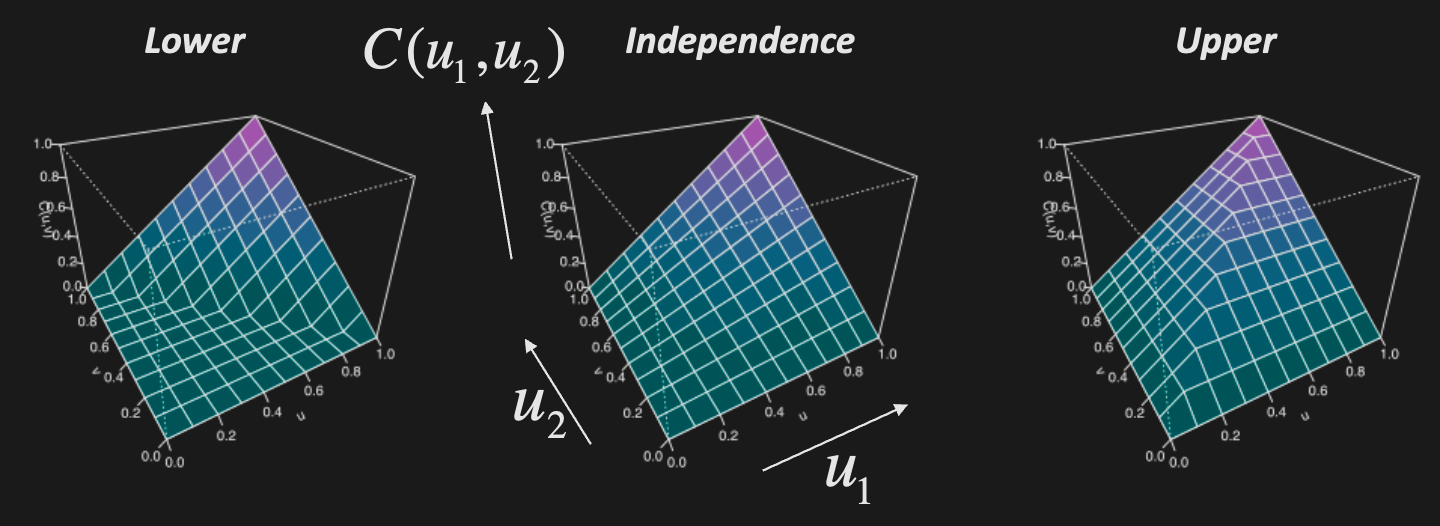
Sklar’s Theorem §

Any continuous multivariate CDF $F(x_1,...,x_d)$ with marginal CDF’s $F_i(x_i),\forall i=1,...,d$ can be expressed as a copula

$$F(x_1,...,x_d)=C(F_1(x_1),...,F_d(x_d))$$

The inverse is also true: any copula combined with marginal CDFs gives a multivariate CDF

If we let $u_i=F_i(x_i)⟹x_i=F_i^{-1}(u_i)⟹C(u_1,...,u_d)=F(F_i^{-1}(u_i),...,F_d^{-1}(u_d))$

So, for continuous CDF $F(x_1,..,x_d)$ with marginals $F_i(x_i)$, the copula is given by

$$C(u_1,...,u_d)=F(F_1^{-1}(u_1),...,F_d^{-1}(u_d))$$

E.g. If $X\sim F$, then $F(X)\sim Unif(0,1)$, and $F^{-1}(Unif)=X\sim F$

Gaussian Copula §

Suppose $\mathbf{X}\sim N_d(\mu ,\mathbf{\Sigma })$ with correlation matrix $\rho$. Its copula is given by

$$C_{\rho }(u_1,...,u_2)={\Phi }_{\mu ,\Sigma }({\Phi }_{{\mu }_1,{\sigma }_1^2}^{-1}(u_1),...,{\Phi }_{{\mu }_d,{\sigma }_d^2}^{-1}(u_d))$$

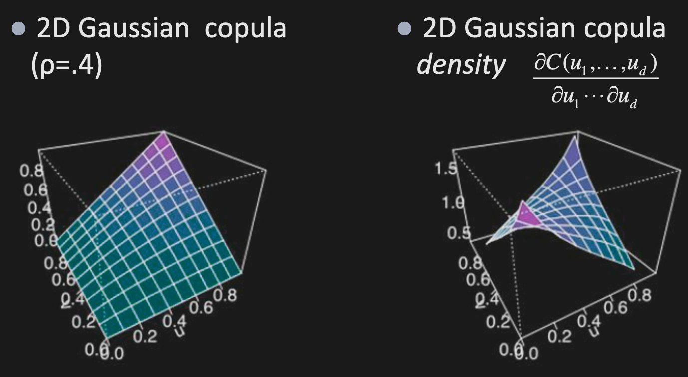
For the independent copula, the derivative would be a plane.

Note: The Gaussian copula only depends on $\rho$, not on the individual means and variances (${\mu }_i$’s and $\sigma$’s). Shown below.

$$\begin{array}{rl}{C}_{Gaussian}(u_1,\dots ,u_d)& ={\Phi }_{\mu ,\Sigma }({\Phi }_{{\mu }_1,{\sigma }_1^2}^{-1}(u_1)...,{\Phi }_{{\mu }_2,{\sigma }_2^2}^{-1}(u_2))\\ & ={\Phi }_{\mu ,\Sigma }\left({\mu }_1+{\sigma }_1{\Phi }_{0,1}^{-1}(u_1),\dots ,{\mu }_d+{\sigma }_d{\Phi }_{0,1}^{-1}(u_d)\right)\\ & ={\Phi }_{0,\varphi }\left(\frac{[{\mu }_1+{\sigma }_1{\Phi }_{0,1}^{-1}(u_1)]-{\mu }_1}{{\sigma }_1},\dots ,\frac{[{\mu }_d+{\sigma }_d{\Phi }_{0,1}^{-1}(u_d)]-{\mu }_d}{{\sigma }_d}\right)\\ & ={\Sigma }_{0,\varphi }({\Phi }_{0,1}^{-1}(u_1),\dots ,{\Phi }_{0,1}^{-1}(u_d))\end{array}$$

Meta-Gaussian distributions §

Multivariate distributions with a Gaussian copula

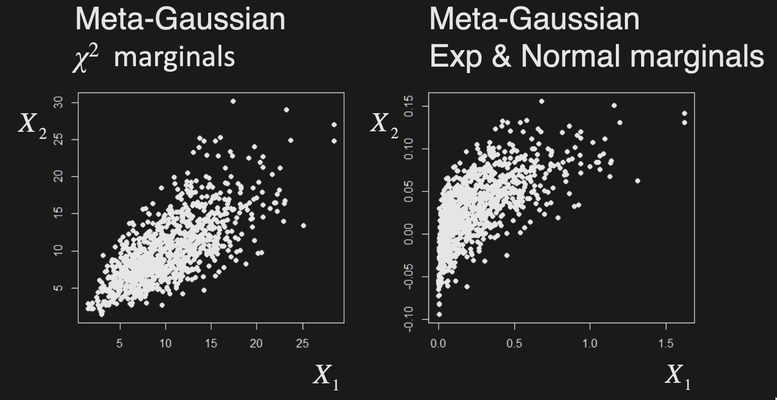
Simulation §

Copulas can be created from known distributions. To simulate data from a distribution with copula $C$ and marginals $F_i$:

1. Generate (dependent) uniforms

$$(U_1,...,U_d)\sim C$$

2. Generate target variates from marginals

$$X_i=F_i^{-1}(U_i)\forall i$$

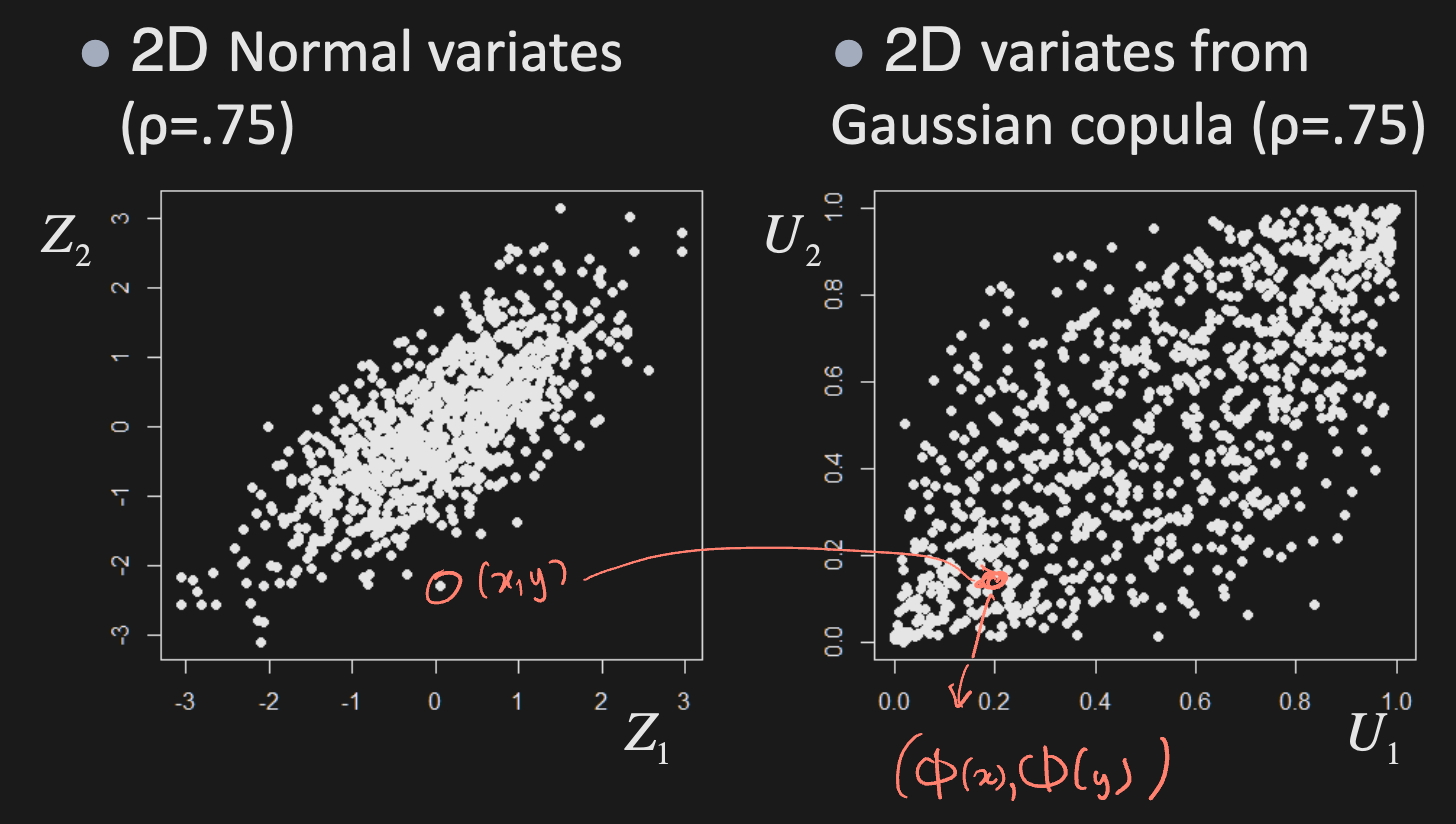
E.g. To generate uniforms from Gaussian copula:

1. Generate multivariate normals with correlation $\rho$

$$\mathbf{Z}\sim N_d(0,\mathbf{\rho })$$

2. Calculate uniforms as their marginal CDF’s

$$U_i=\Phi (Z_i)$$

3. Then, use these uniforms with any other marginals

For $\rho =0$, the pdf of a Gaussian copula vs a t copula looks like

Elliptical copula §

Normal and t distributions both have a dependence structure that is said to be elliptical (due to their elliptical contours)

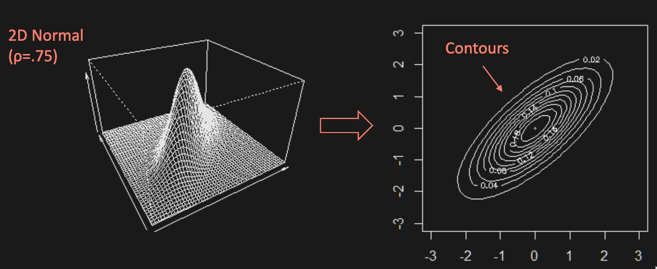
Symmetry of covariance matrix $⟺$ same dependence strength for positively and negatively correlated values

Archimedean copula §

Family of copulas with the following form

$$C(u_1,\dots ,u_d)={\varphi }^{-1}(\varphi (u_1)+\cdots +\varphi (u_d))$$

where $\varphi$ is called the generator function with the following properties:

• $\varphi$ is continuous and convex
• $\varphi :[0,1]\to [0,\infty ]$
• $\varphi (0)=\infty ,\varphi (1)=0$

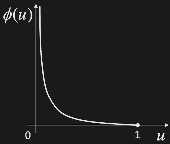
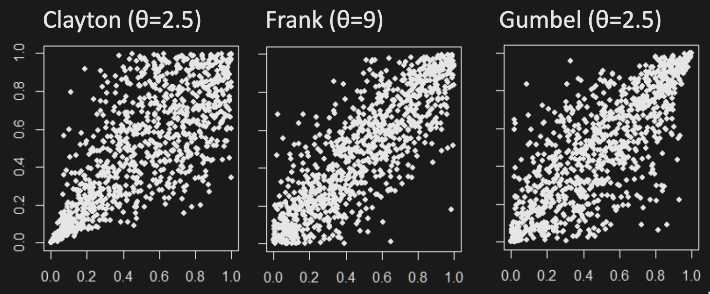
There are infinitely many choices for $\varphi$, but the most common ones are:

$$\begin{array}{lccc}\text{ Name }& \text{ Generator }\varphi (t)& \text{ Generator Inverse }{\varphi }^{-1}(s)& \text{ Parameter }\\ \text{ Clayton }& t^{-\theta }-1& (1+s{)}^{-1/\theta }& \theta \ge 0\\ \text{ Frank }& -\ln \frac{e^{-\theta t}-1}{e^{-\theta }-1}& -\frac{1}{\theta }\ln \left(1+e^{-s}\left(e^{-\theta }-1\right)\right)& \theta \ge 0\\ \text{ Gumbel }& (-\ln t{)}^{\theta }& e^{-\theta \cdot \sqrt{s}}& \theta \ge 1\end{array}$$

2D Archimedean copula random variates:

Contours of 2D pdf’s with Archimedean copulas and standard normal marginals:

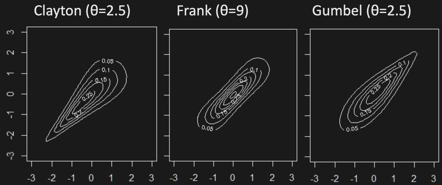
Although Archimedean copulas can model dependence asymmetries, there are limitations in $\ge$ 3D

• The copula value is constant for any permutation of coordinates $u_1,\dots ,u_d$

$$C(u_1,\dots ,u_d)={\varphi }^{-1}(\varphi (u_1)+\cdots +\varphi (u_d)$$

• All pairs of coordinates have the same dependence, which is not the case for elliptical copulas

Alternative: vine copulas, which allow for both asymmetry and differences in pairwise dependence.

Fitting copulas §

For given copula and marginals, we can use MLE to fit multivariate distribution parameters to data, but the number of parameters can be very high.

Instead, use pseudo-MLE to break problem down into marginals and copula:

• Estimate marginal params for each dimension and calculate uniforms

$$U_i^{(j)}=\widehat{F_j}(X_i^{(j)}),\forall i=1,\dots ,n,j=1,\dots ,d$$

• Then estimate copula using ML on uniforms

W4: Portfolio Theory §

Assumptions:

• Static multivariate return distribution
• Investors have same views on mean & variance
• Investors want minimum risk for maximum return
• Investors measure risk by portfolio’s variance
• No borrowing or short-selling restrictions
• No transaction costs

Two asset portfolio §

The portfolio return is $R_p=w_1{R}_1+w_2{R}_2$

$$\begin{array}{rl}{R}_p& =\frac{V(t)-V(0)}{V(0)}\\ & =\frac{(x_1{S}_1(t)+x_2{S}_2(t))-(x_1{S}_1(0)+x_2{S}_2(0))}{V(0)}\\ & =\frac{x_1(S_1(t)-S_1(0))+x_2(S_2(t)-S_2(0))}{V(0)}\\ & =x_1\underset{R_1}{\underbrace{\frac{S_1(t)-S_1(0)}{S_1(0)}}}\frac{S_1(0)}{V(0)}+x_2\underset{R_2}{\underbrace{\frac{S_2(t)-S_2(0)}{S_2(0)}}}\frac{S_2(0)}{V(0)}\\ & =\underset{w_1}{\underbrace{\frac{x_1{S}_1(0)}{V(0)}}}{R}_1+\underset{w_2}{\underbrace{\frac{x_2{S}_2(0)}{V(0)}}}{R}_2\end{array}$$

We can model it like so

$$R_p={\mathbf{w}}^T\cdot \mathbf{R}=\left(\begin{array}{cc}{w}_1& w_2\end{array}\right)\left(\begin{array}{c}{R}_1\\ R_2\end{array}\right)$$

where $\mathbf{R}\sim N_2(\mu ,\mathbf{\Sigma })⟹R\sim N_1({\mu }_p,{\sigma }_p^2)$ with

$$\begin{array}{rl}{\mu }_p& =E(R_p)=E({\mathbf{w}}^T\mathbf{R})={\mathbf{w}}^{T}E(\mathbf{R})={\mathbf{w}}^T\mu \\ {\sigma }_p^2& =V(R_p)=V({\mathbf{w}}^T\mathbf{R})={\mathbf{w}}^{T}V(\mathbf{R})\mathbf{w}={\mathbf{w}}^T\Sigma \mathbf{w}\\ & =\left[\begin{array}{cc}{w}_1& w_2\end{array}\right]\left[\begin{array}{cc}{\sigma }_1^2& {\sigma }_{12}\\ {\sigma }_{21}& {\sigma }_2^2\end{array}\right]\left[\begin{array}{c}{w}_1\\ w_2\end{array}\right]\\ & =w_1^2{\sigma }_1^2+2w_1{w}_2{\sigma }_{12}+w_2^2{\sigma }_2^2\end{array}$$

Let $w_1=w$, $w_2=1-w$, then ${\sigma }_p^2=w^2{\sigma }_1^2+2w(1-w){\sigma }_{12}+(1-w{)}^2{\sigma }_2^2$

To minimize, differentiate w.r.t. w and set to 0: $\frac{\partial }{\partial w}{\sigma }_p^2=0$

$$\begin{array}{rl}2w{\sigma }_1^2+2(1-w){\sigma }_{12}-2w{\sigma }_{12}-2(1-w){\sigma }_2^2& =0\\ w({\sigma }_1^2-{\sigma }_{12})+(1-w)({\sigma }_{12}-{\sigma }_2^2)& =0\\ w& =\frac{-{\sigma }_{12}+{\sigma }_2^2}{{\sigma }_1^2+{\sigma }_2^2-2{\sigma }_{12}}\end{array}$$

Multiple asset portfolio §

Consider n risky assets with returns $R_1,\dots ,R_n$

$$\mathbf{R}=\left[\begin{array}{c}{R}_1\\ ⋮\\ R_n\end{array}\right]\sim N\left(\mathbf{\mu }=\left[\begin{array}{c}{\mu }_1\\ ⋮\\ {\mu }_n\end{array}\right],\mathbf{\Sigma }=\left[\begin{array}{ccc}{\sigma }_1^2& \cdots & {\sigma }_{1n}\\ ⋮& \ddots & ⋮\\ {\sigma }_{n1}& \cdots & {\sigma }_n^2\end{array}\right]\right)$$

A portfolio with weights $\mathbf{w}=[w_1,\dots ,w_n{]}^T$ s.t. ${\sum }_{i=1}^n{w}_i={\mathbf{w}}^{T}1=1$ has

$$R_p\sim N_1({\mu }_p,{\sigma }_p^2)$$

To find the min variance portfolio with given expected return ${\mu }_p$, we solve the following quadratic optimization problem with linear constraints

$$\underset{\mathbf{w}}{\min }\left\{{\mathbf{w}}^{\top }\mathbf{\Sigma }\mathbf{w}\right\}\text{, subject to }\{\begin{array}{l}{\mathbf{w}}^{\top }\mathbf{\mu }={\mu }_p\\ {\mathbf{w}}^{\top }1=1\end{array}$$

The set of such portfolios forms a parabola in mean-variance space, containing attainable portfolios.

Minimum variance portfolio weights §

We can use Lagrange multipliers to find the minimum variance portfolio weights:

Lagrange Multipliers are used to find the local max/min subject to equality constraints

1 constraint (2 variables): example

$$\begin{array}{rl}\mathcal{L}(x,y,\lambda )& =f(x,y)-\lambda g(x,y)\\ {\nabla }_{x,y,\lambda }\mathcal{L}(x,y,\lambda )& =0⟺\{\begin{array}{l}{\nabla }_{x,y}f(x,y)=\lambda {\nabla }_{x,y}g(x,y)\\ g(x,y)=0\end{array}\end{array}$$

M constraints (n variables):

$$\begin{array}{rl}\mathcal{L}\left(x_1,\dots ,x_n,{\lambda }_1,\dots ,{\lambda }_M\right)& =f\left(x_1,\dots ,x_n\right)-\sum _{k=1}^M{\lambda }_k{g}_k\left(x_1,\dots ,x_n\right)\\ {\nabla }_{x_1,\dots ,x_n,{\lambda }_1,\dots ,{\lambda }_M}\mathcal{L}\left(x_1,\dots ,x_n,{\lambda }_1,\dots ,{\lambda }_M\right)& =0⟺\{\begin{array}{l}\nabla f(\mathbf{x})-{\sum }_{k=1}^M{\lambda }_k\nabla g_k(\mathbf{x})=0\\ g_1(\mathbf{x})=\cdots =g_M(\mathbf{x})=0\end{array}\end{array}$$

Objective function (Lagrangian):

$$L(\mathbf{w},\lambda )={\mathbf{w}}^T\mathbf{\Sigma w}-\lambda ({\mathbf{w}}^{T}1-1)$$

Differentiate and set to 0:

$$\begin{array}{rl}\frac{\partial \mathbf{L}}{\partial \mathbf{w}}& =0\\ 2\mathbf{\Sigma w}-\lambda 1& =0\\ \mathbf{w}& =\frac{\lambda }{2}{\mathbf{\Sigma }}^{-1}1\end{array}$$

Solve for lambda:

$${\mathbf{w}}^{T}1=1⟹\frac{\lambda }{2}\cdot 1^T{\mathbf{\Sigma }}^{-1}1=1⟹\lambda =\frac{2}{1^T{\mathbf{\Sigma }}^{-1}1}$$

Plugging lambda into $\mathbf{w}$, we get

$${\mathbf{w}}^{\ast }=\frac{{\mathbf{\Sigma }}^{-1}1}{1^T{\mathbf{\Sigma }}^{-1}1}$$

It is the row sums of ${\Sigma }^{-1}$ divided by the sum of all its elements.

Risk-free asset §

Consider splitting an investment into portfolio $\left({\mu }_p,{\sigma }_p\right)$ & risk-free asset, with weights $w_p$ and $1-w_p$

A risk-free asset has constant return $R_f={\mu }_f>0,{\sigma }_f=0$

The return is given by $R=w_p{R}_p+(1-w_p)R_f$, with

• $E(R)=w_{p}E(R_p)+(1-w_p)E(R_p)=w_p{\mu }_p+(1-w_p){\mu }_f$
• $V(R)=V(w_p{R}_p+(1-w_p)R_f)=w_p^{2}V(R_p)=w_p^2{\sigma }_p^2$

For a set of assets including risk-free ones, the best investments lie on the line tangent to the efficient frontier - they are combinations of the tangency portfolio and risk free assets.

• The tangency portfolio is the efficient frontier portfolio that belongs to the tangent line.
• The slope of the line is the Sharpe ratio.

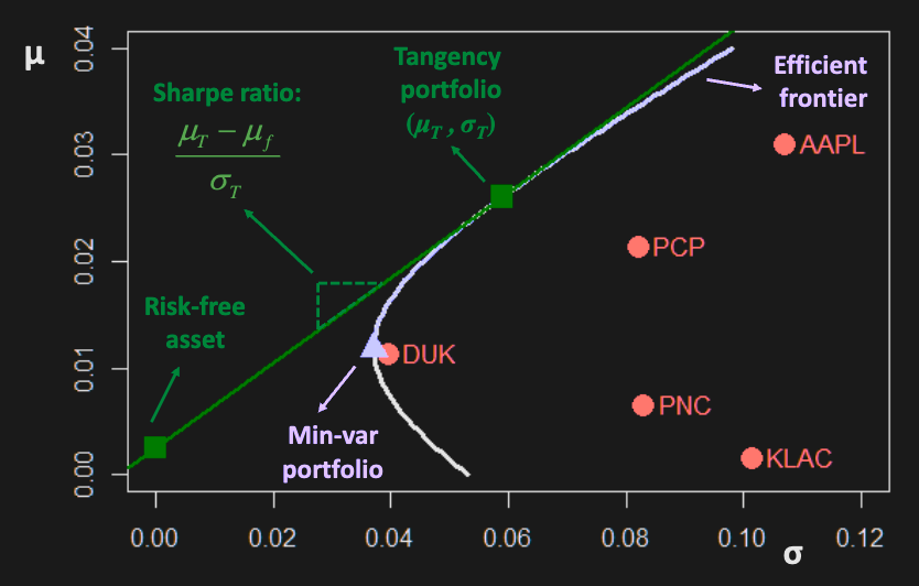
To find the tangency portfolio, maximize Sharpe ratio.

$$\max \left\{\frac{{\mu }_p-{\mu }_f}{{\sigma }_p}\right\}=\underset{\mathbf{w}}{\max }\left\{\frac{{\mathbf{w}}^{\top }\mathbf{\mu }-{\mu }_f}{\sqrt{{\mathbf{w}}^{\top }\mathbf{\Sigma }\mathbf{w}}}\right\},\text{ subject to }{\mathbf{w}}^{\top }1=1$$

Tangency portfolio weights (solution to above) are given by

$${\mathbf{w}}_T=\frac{{\mathbf{\Sigma }}^{-1}\left(\mathbf{\mu }-{\mu }_f\right)}{1^{\top }{\mathbf{\Sigma }}^{-1}\left(\mathbf{\mu }-{\mu }_f\right)}$$

CAPM (Capital asset pricing model) §

If every investor follows mean-variance analysis & the market is in equilibrium, then:

1. Every investor holds some portion of the same tangency portfolio
2. The entire financial market is composed of the same mix of
   risky assets
3. Tangency portfolio is simply the market value-weighted index

Market portfolio §

Since composition of the tangency portfolio is equivalent to that of the market portfolio, its weights are just

$$w_i=\frac{S_i{O}_i}{{\sum }_{i=1}^N{S}_i{O}_i}$$

where $S_i$ = price of asset i, $O_i$ = # shares outstanding

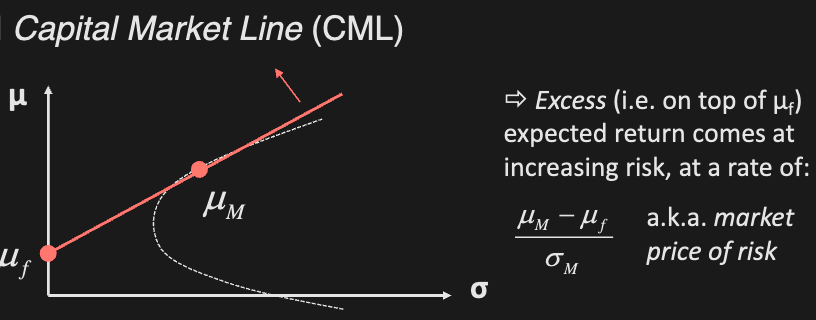
Capital market line §

Every mean-variance efficient portfolio $({\mu }_p,{\sigma }_p)$ lies on the capital market line:

$${\mu }_p={\mu }_f+\frac{{\mu }_M-{\mu }_f}{{\sigma }_M}{\sigma }_p$$

where ${\mu }_f$ is the risk free rate, and $({\mu }_M,{\sigma }_M)$ is the market portfolio

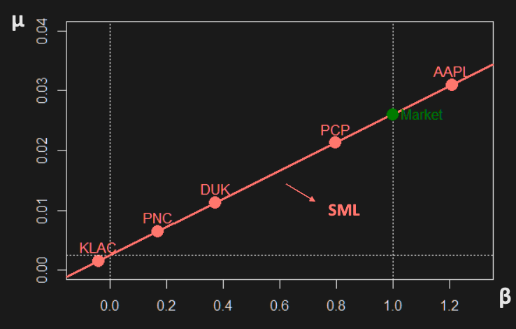
Security market Line §

CAPM implies the following relationship between risk and expected return for all assets/portfolios (not just efficient ones)

$$\begin{array}{rl}{\mu }_i& ={\mu }_f+{\beta }_i({\mu }_M-{\mu }_f)\text{ where }{\beta }_i=\frac{{\sigma }_{iM}}{{\sigma }_M^2}=\frac{Cov(R_i,R_M)}{{\sigma }_M^2}\\ & ={\mu }_f+{\beta }_i\underset{\text{Sharpe Ratio}}{\underbrace{\left(\frac{{\mu }_M-{\mu }_f}{{\sigma }_M}\right)}}{\sigma }_M\end{array}$$

Implications:

• At equilibrium, an asset’s return depends only on its relation to the market portfolio.
  • ${\beta }_i$ measures the extent to which an asset’s return is related to the market. Higher $|\beta |⟺$ higher risk and reward.
• Investors are only rewarded with higher returns for taking on market/systematic risk

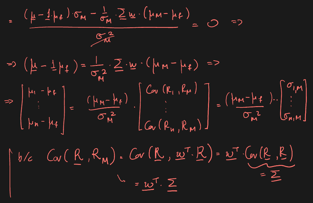
Derivation: max Sharpe ratio using 1st order conditions

$$\underset{\mathbf{w}}{\max }\left\{\frac{{\mu }_M-{\mu }_f}{{\sigma }_M}\right\}=\underset{\mathbf{w}}{\max }\left\{\frac{{\mathbf{w}}^{\top }\mathbf{\mu }-{\mu }_f}{\sqrt{{\mathbf{w}}^{\top }\mathbf{\Sigma }\mathbf{w}}}\right\}\text{, subject to }{\mathbf{w}}^{\top }1=1$$

E.g. Consider N assets with iid $N(\mu ,{\sigma }^2)$ returns and risk free return ${\mu }_f<\mu$. Find market portfolio weights and SML.

$\forall \mathbf{w}\text{ s.t. }{\mathbf{w}}^{T}1=1$, ${\mathbf{w}}^T\mu 1=\mu$

Since the market portfolio is the min variance portfolio, we have

$${\mathbf{w}}^{\ast }=\frac{{\mathbf{\Sigma }}^{-1}1}{1^T{\mathbf{\Sigma }}^{-1}1}=\frac{\frac{1}{{\sigma }^2}I1}{\frac{1}{{\sigma }^2}{1}^{T}I1}=\frac{1}{N}⟹w_i=\frac{1}{N},\forall i=1,\dots ,N$$

So the minimum variance is

$${\mathbf{w}}^T\mathbf{\Sigma }\mathbf{w}={\left(\frac{1}{N}\right)}^2{1}^T({\sigma }^2\mathbf{I})1={\sigma }^2\frac{1}{N^2}N=\frac{{\sigma }^2}{N}$$

Security characteristic line §

To find ${\beta }_i$’s empirically, regress ($R_i-R_f$) on ($R_M-R_f$)

$$(R_{i,t}-R_{f,t})={\beta }_i(R_{M,t}-R_{f,t})+{ϵ}_t,\text{ where }{ϵ}_t\sim N(0,{\sigma }_{ϵ,i}^2)$$

• $R_M$ is the market return (proxy by large market index, ex S&P500)
• $R_f$ is the risk free rate (proxy by T-bill)

The slope of the SCL is the beta estimate:

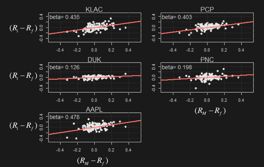
Mean return vs estimated betas:

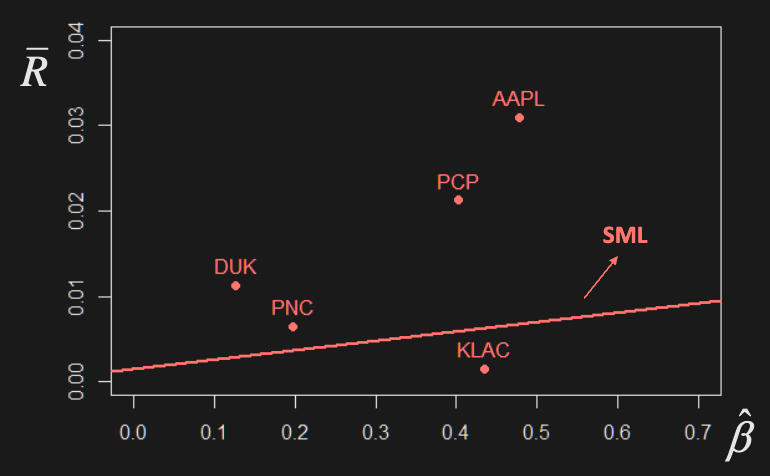
Now consider adding an intercept, $\alpha$

$$(R_{i,t}-R_{f,t})={\alpha }_i+{\beta }_i(R_{M,t}-R_{f,t})+{ϵ}_t$$

The mean and variance are given by

$$\begin{array}{rl}{\mu }_i=E[R_i]& =E[R_{f,t}+{\alpha }_i+{\beta }_i(R_{M,t}-R_{f,t})+{ϵ}_t]\\ & =\underset{R_f}{\underbrace{E[R_f]}}+{\alpha }_i+{\beta }_i\underset{{\mu }_{m-R_f}}{\underbrace{E[R_m-R_f]}}+\underset{=0}{\underbrace{E[{ϵ}_t]}}\\ & =R_f+{\alpha }_i+{\beta }_i({\mu }_m-R_f)\\ & \\ {\sigma }_i^2=\mathbb{V}[R_i]& =\mathbb{V}[\underset{Var=0}{\underbrace{R_f+{\alpha }_i}}+{\beta }_i(R_m-R_f)+{ϵ}_i)]\\ & =\mathbb{V}[{\beta }_i(R_m-\underset{Var=0}{\underbrace{R_f}})]+\mathbb{V}[{ϵ}_i]\\ & ={\beta }_i^2\cdot \mathbb{V}[R_M]+{\sigma }_{ϵ,i}^2\\ & ={\beta }_i^2\cdot {\sigma }_m^2+{\sigma }_{ϵ,i}^2\end{array}$$

${\alpha }_i$ measures the excess increase in asset return on top of that explained by the ${\beta }_i$. The bigger the alpha, the higher the outperformance (compared to the market portfolio).

Legacy of CAPM §

CAPM says the best portfolio you can create is the tangency/market portfolio. This implies the best you can do is get the broadest index and combine it with a T-bill.

CAPM is wrong, but had immense practical impact on investing, specifically in terms of

• Diversification: concept of decreasing risk by spreading portfolio over different assets

• Index investing: justification for common investing strategy of tracking some broad index with mutual funds or ETF’s

• Benchmarking: Measuring performance of investment relative to market / index

Performance Evaluation §

There are several ways to measure an asset’s performance, based on CAPM

Sharpe ratio: (excess return per unit risk)

$$S_i=\frac{{\mu }_i-{\mu }_f}{{\sigma }_i}$$

Treynor index: (excess return per unit non-diversifiable risk)

$$T_i=\frac{{\mu }_i-{\mu }_f}{{\beta }_i}$$

Jensen’s alpha: (excess return on top of the return explained by the market)

$${\alpha }_i={\hat{\alpha }}_i$$

• Usually the most important measure a portfolio manager tries to use to convince people to invest in them.

W5: Factor Models §

Main implication of CAPM: the market is the single factor driving asset returns

To improve performance, use more factors that drive asset returns

Factor Models §

3 types:

1. Macroeconomic: Factors are observable economic and financial time series
2. Fundamental: Factors are created from observable asset characteristics
3. Statistical: Factors are unobservable, and extracted from asset returns

All 3 types follow some form of

$$R_i(t)={\beta }_{i,0}+{\beta }_{i,1}{F}_1(t)+\cdots +{\beta }_{i,p}{F}_p(t)+{ϵ}_i(t),\forall \{\begin{array}{l}i=1,\dots ,N\\ t\in \mathbb{R}\end{array}$$

• $R_i(t)$ is return on the $i^{th}$ asset at time t
• $F_j(t)$ is the $j^{th}$ common factor at time t
• ${\beta }_{i,j}$ is the factor loading/beta of $i^{th}$ asset on the $j^{th}$ factor
• ${ϵ}_i(t)$ is the idiosyncratic/unique return of asset $i^{th}$

In matrix form:

$$\begin{array}{rl}\left[\begin{array}{c}{R}_1(t)\\ ⋮\\ R_N(t)\end{array}\right]& =\left[\begin{array}{c}{\beta }_{1,0}\\ ⋮\\ {\beta }_{N,0}\end{array}\right]+\left[\begin{array}{ccc}{\beta }_{1,1}& \cdots & {\beta }_{1,p}\\ ⋮& \ddots & ⋮\\ {\beta }_{N,1}& \cdots & {\beta }_{N,p}\end{array}\right]\left[\begin{array}{c}{F}_1(t)\\ ⋮\\ F_p(t)\end{array}\right]+\left[\begin{array}{c}{\epsilon }_1(t)\\ ⋮\\ {\epsilon }_p(t)\end{array}\right]\\ & \iff \\ \mathbf{R}(t)& ={\mathbf{\beta }}_0+{\mathbf{\beta }}^{\top }\mathbf{F}(t)+\mathbf{\epsilon }(t)\end{array}$$

Assumptions:

• Asset specific errors ${ϵ}_i$ are uncorrelated with common factors

$$Cov(\mathbf{ϵ}(t),\mathbf{F}(t))=0$$

• The factors $F_j(t)$ are stationary, with moments

$$E(\mathbf{F}(t))={\mathbf{\mu }}_F,\mathbb{V}(\mathbf{F}(t))={\mathbf{\Sigma }}_F$$

• Errors are serially and contemporaneously uncorrelated across assets

$$\begin{array}{rl}E(ϵ)& =0\\ \mathbb{V}(\mathbf{ϵ}(t))& =\text{diag}[{\left\{{\sigma }_{{ϵ}_i}^2\right\}}_{i=1,\dots ,N}]={\Sigma }_{ϵ}\\ Cov[\mathbf{ϵ}(t),\mathbf{ϵ}(s)]& =0\end{array}$$

Find moments of model $\mathbf{R}(t)={\mathbf{\beta }}_0+{\mathbf{\beta }}^T\mathbf{F}(t)+\mathbf{ϵ}(t)$

$$\begin{array}{rl}{\mu }_R& =E({\beta }_0+{\beta }^{T}F(t)+ϵ(t))\\ & ={\beta }_0+{\beta }^{T}E(F(t))+E(ϵ(t))\\ & ={\beta }_0+{\beta }^T{\mu }_F\\ {\Sigma }_R& =V({\beta }_0+{\beta }^{T}F(t)+ϵ(t))\\ & =V({\beta }^{T}F(t))+V(ϵ(t))\\ & ={\beta }^{T}V(F(t))\beta +{\Sigma }_{ϵ}\\ & ={\beta }^T{\Sigma }_F\beta +{\Sigma }_{ϵ}\end{array}$$

Find moments of portfolio with $\mathbf{w}=[w_1\dots w_N{]}^T$, i.e. $R={\mathbf{w}}^T\mathbf{R}$

$$\begin{array}{rl}\mu & =E(w^{T}R)=w^{T}E(R)=w^T({\beta }_0+\beta {\mu }_F)\\ {\sigma }^2& =V(w^{T}R)=w^{T}V(R)w=w^T({\beta }^T{\Sigma }_F\beta +{\Sigma }_{ϵ})w\end{array}$$

Time Series Regression Models §

Consider model for which factor values are known (e.g. macro/fundamental model).

We can estimate betas & risks (variances) for one asset at a time. For each $i=1,\dots N$, fit regression model:

$$R_i(t)={\beta }_{i,0}+{\beta }_{i,1}{F}_1(t)+\cdots +{\beta }_{i,p}{F}_p(t)+{ϵ}_i(t)$$

over observations $t=1,\dots ,T$

Most models will always include some proxy for the overall economy (e.g. the market). The following is a famous example.

Fama-French 3 Factor Model §

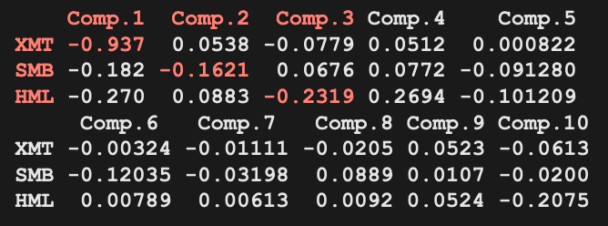
3 factors

• Excess Market Return (XMT)
  • Same as in CAPM.
• Small Minus Big (SMB)
  • Captures the size (market cap) of the company/stock.
• High Minus Low (HML)
  • High = value stock; low = growth stock.
  • Measured using book-to-market ratio.

We can use the factor model to estimate the return covariance matrix.

$$\mathrm{Var}(\mathbf{R})={\hat{\mathbf{\Sigma }}}_R={\hat{\mathbf{\beta }}}^{\top }{\hat{\mathbf{\Sigma }}}_F\hat{\mathbf{\beta }}+{\hat{\mathbf{\Sigma }}}_{\epsilon }$$

where:

$$\begin{array}{rl}& \hat{\mathbf{\beta }}=\text{ beta coefficient matrix (from regressions) }\\ & {\hat{\mathbf{\Sigma }}}_F=\text{ factor sample covariance matrix }\\ & {\hat{\mathbf{\Sigma }}}_{\epsilon }=\text{ diagonal error variance matrix (from residuals) }\end{array}$$

This gives more stable estimates than sample covariance.

Statistical Factor Models §

Factors are unknown and unobserved

• Need to estimate both $\beta$ and $F$
• Problem is ill-posed $⟹$ need constraints

Assumptions §

• Asset specific errors ${ϵ}_i$ are uncorrelated with common factors

$$Cov(\mathbf{ϵ}(t),\mathbf{F}(t))=0$$

• The factors $F_j(t)$ are orthogonal, with moments

$$\begin{array}{rl}E(\mathbf{F}(t))& =0\\ \mathbb{V}(\mathbf{F}(t))& =\mathbf{I}\end{array}$$

• Errors are serially and contemporaneously uncorrelated across assets

$$\begin{array}{rl}E(ϵ)& =0\\ \mathbb{V}(\mathbf{ϵ}(t))& =\text{diag}[{\left\{{\sigma }_{{ϵ}_i}^2\right\}}_{i=1,\dots ,N}]={\Sigma }_{ϵ}\\ Cov[\mathbf{ϵ}(t),\mathbf{ϵ}(s)]& =0\end{array}$$

Resulting moments of returns

$$\begin{array}{rl}{\mu }_R& =E[R]=E[{\beta }_0+{\beta }^{T}F+ϵ]={\beta }_0+{\beta }^T\underset{0}{\underbrace{E[F]}}+\underset{0}{\underbrace{E[ϵ]}}={\beta }_0\\ {\Sigma }_R& =\mathbb{V}[R]=\mathbb{V}[{\mathbf{\beta }}_0+{\mathbf{\beta }}^{T}F+\mathbf{ϵ}]={\mathbf{\beta }}^T\mathbb{V}[F]\mathbf{\beta }+{\mathbf{\Sigma }}_{\mathbf{ϵ}}={\mathbf{\beta }}^{\mathbf{T}}(\mathbf{I}\cdot {\mathbf{\sigma }}_{\mathbf{F}})\mathbf{\beta }+{\mathbf{\Sigma }}_{\mathbf{ϵ}}\end{array}$$

Principal component analysis §

PCA: constructing a set of variables (components) that capture most of the variability given a set of $\mathrm{N}$ assets

It can be thought of as a linear transformation of original variables.

For a random vector $\mathbf{R}={\left[\begin{array}{lll}{R}_1& \cdots & R_N\end{array}\right]}^{\prime }$ with covariance ${\mathbf{\Sigma }}_R$ (correlation ${\mathbf{\rho }}_R$ ), the PC’s are linear combinations of $\left(R_1,\dots ,R_N\right)$

$$\begin{array}{c}{F}_1={\gamma }_1^{\top }\mathbf{R}={\gamma }_{11}{R}_1+\cdots +{\gamma }_{1N}{R}_N\\ ⋮\\ F_N={\mathbf{\gamma }}_N^{\top }\mathbf{R}={\gamma }_{N1}{R}_1+\cdots +{\gamma }_{NN}{R}_N\end{array}$$

such that:

• $F_1,\dots ,F_N$ are uncorrelated
• Each component has maximum variance

Problem definition

We want to find components $F_i,F_j$ (i.e. find coefficient vectors ${\gamma }_i$) s.t.

• $F_i={\mathbf{\gamma }}_i^{\top }\mathbf{X}$ maximizes $\mathrm{Var}\left(F_i\right)={\mathbf{\gamma }}_i^{\top }{\mathbf{\Sigma }}_R{\gamma }_i$ subject to ${\gamma }_i^{\top }{\gamma }_i=1$
• $Cov\left(F_i,F_j\right)={\mathbf{\gamma }}_i^{\top }{\mathbf{\Sigma }}_R{\gamma }_j=0$, for any $j<i$

Solution

Given by eigen-decomposition of ${\mathbf{\Sigma }}_{\mathrm{R}}$

$${\mathbf{\Sigma }}_R={\lambda }_1{\mathbf{e}}_1{\mathbf{e}}_1^{\top }+\cdots +{\lambda }_N{\mathbf{e}}_N{\mathbf{e}}_N^{\top }=\mathbf{P}\Lambda {\mathbf{P}}^{\top }$$

where

$$\mathbf{P}=\left[\begin{array}{ccc}|& & |\\ {\mathbf{e}}_1& \cdots & {\mathbf{e}}_N\\ |& & |\end{array}\right]\text{ and }\mathbf{\Lambda }=\left[\begin{array}{ccc}{\lambda }_1& \cdots & 0\\ ⋮& \ddots & ⋮\\ 0& \cdots & {\lambda }_N\end{array}\right]$$

• P is an orthogonal matrix, i.e. $P^{-1}=P^T$
• ${\lambda }_1\ge \cdots \ge {\lambda }_N\ge 0$

Principal components: $F_j=e_j^T\mathbf{R}=e_{j_1}{R}_1+\cdots +e_{jN}{R}_N,\forall j=1,\dots ,N$

$$\mathbf{F}={\mathbf{P}}^T\mathbf{R}=\left[\begin{array}{ccc}-& e_1^T& -\\ & ⋮& \\ -& e_N^T& -\end{array}\right]\mathbf{R}$$

Find $Var(\mathbf{F})$

$$\begin{array}{rl}\mathbb{V}(\mathbf{F})& =\mathbb{V}({\mathbf{P}}^T\mathbf{R})\\ & ={\mathbf{P}}^T\mathbb{V}(\mathbf{R})\mathbf{P}\\ & ={\mathbf{P}}^T{\mathbf{\Sigma }}_R\mathbf{P}\\ & ={\mathbf{P}}^{\mathbf{T}}(\mathbf{P\Lambda }{\mathbf{P}}^{\mathbf{T}})\mathbf{P}\\ & =\mathbf{\Lambda }\end{array}$$

Find the loading of $R_i$ on $F_j$ (the beta)

$$\begin{array}{rl}{R}_i& =\sum _{j=1}^N{\beta }_{i,j}{F}_j\text{ where }{\beta }_{i,j}=\frac{Cov(R_j,F_j)}{Var(F_j)}\\ Cov(\mathbf{R},\mathbf{F})& =Cov(\mathbf{R},{\mathbf{P}}^T\mathbf{R})\\ & =Cov(\mathbf{R},\mathbf{R})\mathbf{P}\\ & ={\mathbf{\Sigma }}_R\mathbf{P}\\ & =(P\Lambda P^T)P\\ & =P\Lambda \\ & =P\left[\begin{array}{ccc}{\lambda }_1& & 0\\ & \ddots & \\ 0& & {\lambda }_N\end{array}\right]\\ Var(F_j)& ={\lambda }_j\end{array}$$

Total variance of all PC’s = variance of original variable

$$\begin{array}{rl}tr(\Lambda )& =tr(\Sigma )\\ {\lambda }_1+\cdots +{\lambda }_p& ={\sigma }_1^2+\dots {\sigma }_N^2\end{array}$$

Proportion of total variance explained by each PC is

$$\frac{{\lambda }_j}{{\lambda }_1+\cdots +{\lambda }_N}$$

How do we choose the number of PCs?

• We can use a scree plot:

  

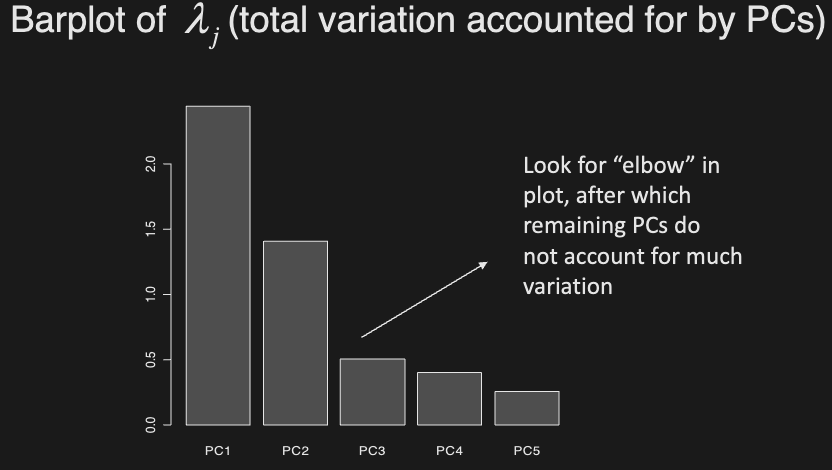
• E.g. In this example, one PC already explains much of the variation

  

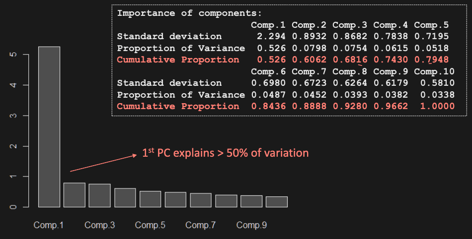
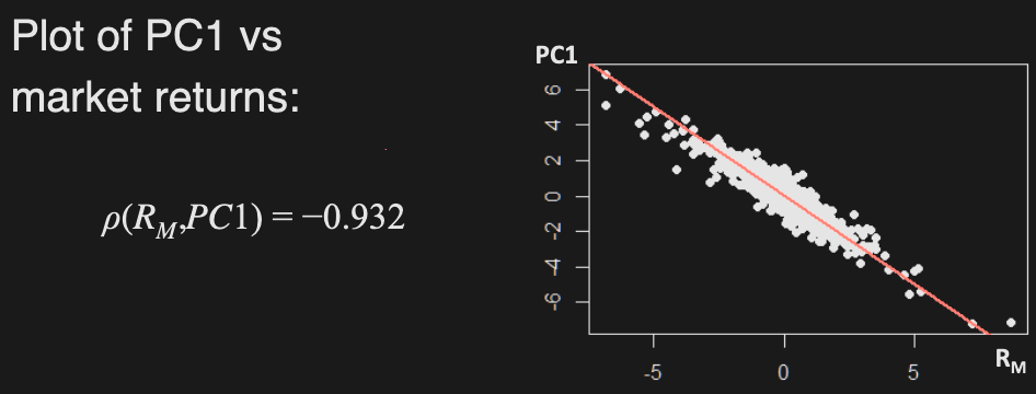
PCA can be used to identify components that explain overall variation of data, but it does not always give meaningful PC’s - PC’s are just transformations that capture the most variability, they do not explain how data was generated.

For a proper data-generating model, use Factor Analysis:

Factor Analysis §

Assuming ${\mathbf{\Sigma }}_F=\mathbf{I}$, the return variance becomes ${\mathbf{\Sigma }}_R=\underset{communality}{\underbrace{{\mathbf{\beta }}^T\mathbf{\beta }}}+\underset{uniqueness}{\underbrace{{\mathbf{\Sigma }}_{ϵ}}}$

We need to estimate $\mathbf{\beta }$ and variances ${\sigma }_{{ϵ}_i}^2$ using maximum likelihood.

A rotation of $\mathbf{\beta }$ (scaling it with orthogonal matrix P) has no effect on the model:

$${\mathbf{\Sigma }}_R=\left({\mathbf{\beta }}^{\top }\mathbf{P}\right)\left({\mathbf{P}}^{\top }\mathbf{\beta }\right)+{\mathbf{\Sigma }}_{\epsilon }={\mathbf{\beta }}^{\top }\left({\mathbf{PP}}^{\top }\right)\mathbf{\beta }+{\mathbf{\Sigma }}_{\epsilon }={\mathbf{\beta }}^{\top }\mathbf{\beta }+{\mathbf{\Sigma }}_{\epsilon }$$

We need further constraints on $\beta$. A common constraint is to rank factors by explained variability, similar to PCA.

W6: Risk Management §

Types of risks §

• Market risk: due to changes in market prices
• Credit risk: counterparty doesn’t honour obligations
• Liquidity risk: lack of asset tradability
• Operational risk: from organization’s internal activities (e.g. legal, fraud, or human error risk)

Risk measures §

• There exists different notions of risk (losing money, bankruptcy, not achieving desired return), but in practice risk measures are used to determine the amount of cash to be kept on reserve

• Return volatility is not a good risk measure. The following distributions have the same $\sigma$, but their risk profiles are very different

  

  • LHS: average return is positive but it has a fat left tail, so returns could be large negative values
  • RHS: average return is negative, but no chance of getting very large negative values; hence less risky

Value at Risk (VaR) §

The VaR is the amount that covers losses with probability $1-\alpha$.

Let $L$ be the loss of an investment over time period $T$. ($L=-R$, where $R$ is revenue).

The VaR is defined as the $1-\alpha$ quantile of $L$ for some $\alpha \in (0,1)$:

$${\mathrm{VaR}}_{\alpha }=\inf \{x:P(L\le x)\ge 1-\alpha \}=\inf \{x:P(L>x)\le \alpha \}$$

For a continuous RV with CDF $F_L$, it is defined as:

$$\begin{array}{rl}Va{R}_{\alpha }& =F_L^{-1}(1-\alpha )\end{array}$$

E.g. Consider asset with $N(\mu =0.03,{\sigma }^2=0.04)$ annual log-returns. Find the 95% confidence level annual VaR for a $1000 investment in this asset.

Want to find VaR($\alpha$) s.t.

$$\begin{array}{rl}P(L>VaR)& =P(-R>VaR)\\ & =P(R<-VaR)\\ & =P(S_T-S_0<-VaR)\\ & =P(S_T<S_0-VaR)\\ & =P(S_0{e}^X<S_0-VaR)\\ & =P\left(X<\log \left(\frac{S_0-VaR}{S_0}\right)\right)\\ & =P\left(\frac{X-0.03}{.2}<\frac{\log \left(1-\frac{VaR}{S_0}\right)-0.03}{.2}\right)\\ 0.05& =P\left(Z<\frac{\log \left(1-\frac{VaR}{S_0}\right)-0.03}{.2}\right)\\ ⟹z=-1.645& =\frac{\log \left(1-\frac{VaR}{S_0}\right)-0.03}{.2}\\ VaR& =(1-\exp \{-1.645\cdot 0.20+0.03\})\cdot S_0\\ & =258.44\end{array}$$

Formula for VaR given log returns:

$$\mathrm{VaR}=S_0(1-\exp \left\{\mu +z\sigma \right\})$$

Limitations §

VaR can be misleading as it hides tail risk and discourages diversification.

However, it is still widely used due to the Basel framework (banking regulations).

As an example, the following have the same VaR but vastly different risk

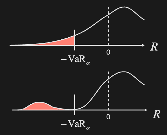
Solution: use conditional VaR / expected shortfall

Conditional VaR / Expected Shortfall §

Defined as the expected value (or average) of losses beyond VaR

$$\frac{1}{\alpha }{\int }_0^{\alpha }VaR(u)du=E(L|L\ge Va{R}_{\alpha })$$

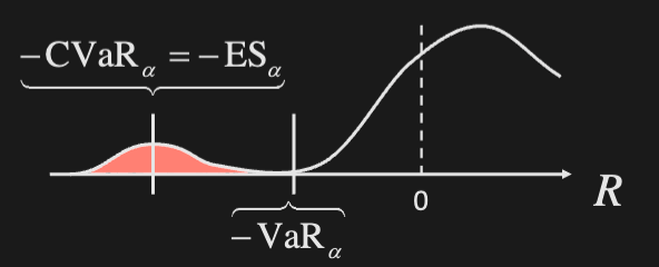
Examples §

VaR & CVaR of a Normal Variable §

If R~N(0, 1), find ES at confidence level $\alpha$

Let $Z_{\alpha }$ denote the top $\alpha$-quantile of the standard normal

Normal pdf:

$$f(x)=\frac{1}{\sqrt{2\pi \sigma }}\exp \left\{-\frac{1}{2}{\left(\frac{x-\mu }{\sigma }\right)}^2\right\}$$

Standard normal pdf:

$$\varphi (x)=\frac{1}{\sqrt{2\pi }}\exp \left\{-\frac{x^2}{2}\right\}$$

$$\begin{array}{rl}E{S}_{\alpha }=E(L|L>z_{\alpha })& ={\int }_{z_{\alpha }}^{\infty }x\varphi (x|L>z_{\alpha })dx\\ & ={\int }_{z_{\alpha }}^{\infty }x\frac{\varphi (x)}{P(L>z_{\alpha })}dx\\ & =\frac{1}{\underset{\alpha }{\underbrace{P(L>z_{\alpha }}})}{\int }_{z_{\alpha }}^{\infty }x\frac{1}{\sqrt{2\pi }}{e}^{-x^2/2}dx\\ & =\frac{1}{\alpha }{\int }_{z_{\alpha }}^{\infty }\frac{1}{\sqrt{2\pi }}[-e^{-x^2/2}{]}^{\prime }dx\\ & =\frac{1}{\alpha }\frac{1}{\sqrt{2\pi }}[-e^{-x^2/2}{]}_{x=z_{\alpha }}^{\infty }\\ & =\frac{1}{\alpha }\frac{1}{\sqrt{2\pi }}{e}^{-z_{\alpha }^2/2}\\ & =\frac{1}{\alpha }\varphi (z_{\alpha })\end{array}$$

More generally, for $L\sim N(\varphi ,{\sigma }^2)$

$$\begin{array}{rl}E{S}_{\alpha }& =\mu +\frac{\varphi (z_{\alpha })}{\alpha }\sigma \\ Va{R}_{\alpha }& =\mu +z_{\alpha }\sigma \end{array}$$

Risk measure properties §

Let $\rho (L)$ denote a risk measure for an investment with loss L.

A coherent risk measure must satisfy the following properties:

1. Normalized (the risk of holding no assets is 0)
   • $\rho (0)=0$
2. Translation invariance (adding loss $c$ to portfolio increases risk by $c$)
   • $\rho (L+c)=\rho (L)+c,\forall c\in \mathbb{R}$
3. Positive homogeneity
   • $\rho (bL)=b\rho (L),\forall b>0$
4. Monotonicity
   • $L_1\ge L_2⟹\rho (L_1)\ge \rho (L_2)$
5. Sub additivity (due to diversification)
   • $\rho (L_1+L_2)\le \rho (L_1)+\rho (L_2)$

E.g. Show that VaR and CVaR are translation invariant and positively homogeneous

Let $L^{\prime }=bL+c$, then

$$\begin{array}{rl}{\mathrm{VaR}}_{\alpha }(L)& =\inf \{x:P(L>x)\le \alpha \}\\ {\mathrm{VaR}}_{\alpha }(L^{\prime })& =\inf \{x^{\prime }:P(L^{\prime }>x^{\prime })\le \alpha \}\\ & =\inf \{x^{\prime }:P(bL+c>x^{\prime })\le \alpha \}\\ & =\inf \left\{x^{\prime }:P\left(L>\frac{x^{\prime }-c}{b}\right)\le \alpha \right\}\\ & =\inf \left\{bx+c:P(L>x)\le \alpha \right\}\\ & =b\inf \left\{x:P(L>x)\le \alpha \right\}+c\\ & =b\mathrm{VaR}(L)+c\end{array}$$

$$\begin{array}{rl}{\mathrm{CVaR}}_{\alpha }(L)& =\frac{1}{\alpha }{\int }_0^{\alpha }{\mathrm{VaR}}_u(L)du\\ {\mathrm{CVaR}}_{\alpha }(L^{\prime })& =\frac{1}{\alpha }{\int }_0^{\alpha }b{\mathrm{VaR}}_u(L)+cdu\\ & =b\left(\frac{1}{\alpha }{\int }_0^{\alpha }Va{R}_u(L)du\right)+c\\ & =b\cdot \mathrm{CVaR}(L)+c\end{array}$$

E.g. Consider 2 risky zero-coupon bonds priced at $95per$100 face value. If each one has 4% independent default probability, show that ${\mathrm{VaR}}_{5\%}$ is not sub-additive.

Distribution of $L_1$ or $L_2$:

$$L_i=\{\begin{array}{ll}-5,& p=96\%\\ 95,& p=4\%\end{array}$$

$$\begin{array}{rl}{\mathrm{VaR}}_{5\%}(L_i)& =\inf \{x:P(L>x)\le 5\%\}\\ & =\inf \{x:P(L\le x)\ge 95\%\}\\ & =-5\end{array}$$

Distribution of $L_1+L_2$:

$$L_1+L_2=\{\begin{array}{ll}-5-5=-10,& p=.96^2=92.15\%\\ -5+95=90,& p=2(.96)(.04)=7.68\%\\ 95+95=190,& p=(.04{)}^2=0.16\%\end{array}$$

$${\mathrm{VaR}}_{5\%}(L_1+L_2)=\inf \{x:P(L_1+L_2\le x)\ge 95\%\}=90$$

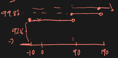
which is greater than

$${\mathrm{VaR}}_{5\%}(L_1)+{\mathrm{VaR}}_{5\%}(L_2)=-5-5=-10$$

This shows that under VaR, owning both bonds is riskier than owning them separately. VaR is thus incoherent at the 5% level (it hides tail risk). At 3%, it would be coherent.

E.g. Show that ${\mathrm{CVaR}}_{5\%}$ is sub-additive.

$$\begin{array}{rl}{\mathrm{CVaR}}_{5\%}(L_1)& =\frac{1}{5\%}{\int }_0^{5\%}{\mathrm{VaR}}_u(L_1)du=\frac{1}{5\%}(95\cdot 4\%+(-5)\cdot 1\%)=73\\ {\mathrm{CVaR}}_{5\%}(L_1+L_2)& =\frac{1}{5\%}{\int }_0^{5\%}{\mathrm{VaR}}_u(L_1+L_2)du=\frac{1}{5\%}(190\cdot 16\%+90\cdot 4.84\%)=93.2\end{array}$$

We see that ${\mathrm{CVaR}}_{5\%}(L_1+L_2)=93.2\le {\mathrm{CVaR}}_{5\%}(L_1)+{\mathrm{CVaR}}_{5\%}(L_2)=2\cdot 73$

Entropic VaR §

EVaR is a coherent alternative to VaR based on the Chernoff bound, which is attained by applying Markov’s inequality to $e^{tX}$. It is an exponentially decreasing upper bound on the tail of a RV based on its MGF.

Markov inequality: for a positive RV $X$, we have

$$P(X\ge c)\le \frac{E(X)}{c},\forall c>0$$

For loss RV $L$ with MGF $M_L(z)=E(e^{zL})<\infty ,\forall z>0$, we have

$$P(L\ge c)=P(e^{zL}\ge e^{zc})\le \frac{M_L(z)}{e^{zc}}$$

Bound this by $\alpha$ and solve for $c$:

$$M_L(z)e^{-zc}\le \alpha ⟹c=z^{-1}\ln (\frac{M_L(z)}{\alpha })$$

Thus, EVaR is defined as

$${\mathrm{EVaR}}_{\alpha }=\underset{z>0}{\inf }\left\{z^{-1}\ln (\frac{M_L(z)}{\alpha })\right\}$$

EVaR of a Normal Variable §

The MGF of a Normal variable $L\sim N(\mu ,{\sigma }^2)$ is

$$\begin{array}{r}{M}_L(Z)=e^{\mu z+\frac{1}{2}{\sigma }^2{z}^2}=E(e^{zL}),\forall z\end{array}$$

EVaR is the infimum of the following:

$$\begin{array}{rl}{z}^{-1}\ln \left(\frac{M_L(z)}{\alpha }\right)& =\frac{1}{z}\ln \left(\frac{e^{\mu z+\frac{1}{2}{\sigma }^2{z}^2}}{\alpha }\right)\\ & =\frac{1}{z}\left(\mu z+\frac{{\sigma }^2{z}^2}{2}-\ln \alpha \right)\\ & =\mu +z\frac{{\sigma }^2}{2}-\frac{\ln \alpha }{z}=f(z)\end{array}$$

To find infimum (minimum) over z>0, differentiate and set to 0:

$$\begin{array}{rl}0& =\frac{{\sigma }^2}{2}+\ln \alpha \left(\frac{1}{z^2}\right)\\ z^{\ast }& =\frac{\sqrt{-2\ln \alpha }}{\sigma }\end{array}$$

So we have

$$\begin{array}{rl}{\mathrm{EVaR}}_{\alpha }(L)& =\underset{z>0}{\inf }\left\{f(z)\right\}=f(z^{\ast })\\ & =\mu +\frac{\sqrt{-2\ln \alpha }}{\sigma }\frac{{\sigma }^2}{2}-\frac{\ln \alpha }{\frac{\sqrt{-2\ln \alpha }}{\sigma }}\\ & =\mu +\frac{\sqrt{-2\ln \alpha }}{\sigma }\frac{{\sigma }^2}{2}+\sigma \frac{\ln {\alpha }^{-1}}{\sqrt{2\ln {\alpha }^{-1}}}\\ & =\mu +\sigma \sqrt{-\frac{\ln \alpha }{2}}+\sigma \sqrt{\frac{\ln {\alpha }^{-1}}{2}}\\ & =\mu +2\sigma \sqrt{\frac{\ln {\alpha }^{-1}}{2}}\\ & =\mu +\sigma \sqrt{2\ln {\alpha }^{-1}}\end{array}$$

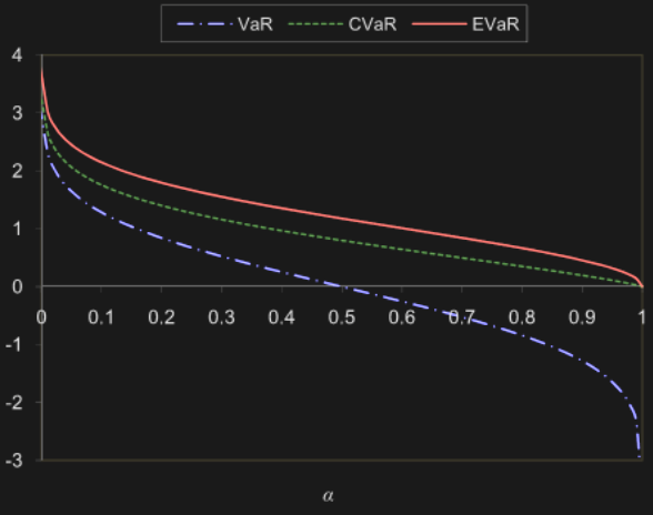
Calculating risk measures §

3 ways:

• Parametric modeling
• Historical simulation
• Monte Carlo simulation

Other risk management techniques: stress-testing (worst-cast scenario) and extreme value theory (EVT)

~85% of large banks use historical simulation, the remaining use MC simulation

Parametric modeling §

Fitting a distribution to revenues/returns and calculating VaR or CVaR/ES based on distribution

E.g. Assuming net returns of an investment follow a normal distribution, then for an initial capital $S_0$, the parametric VaR and CVaR at confidence $1-\alpha$ are

$$\begin{array}{rl}{\mathrm{VaR}}_{\alpha }& =-S_0\times \left\{\hat{\mu }+\hat{\sigma }{\Phi }^{-1}(\alpha )\right\}\\ {\mathrm{CVaR}}_{\alpha }& =-S_0\times \left\{\hat{\mu }+\hat{\sigma }\frac{\varphi \left({\Phi }^{-1}(\alpha )\right)}{\alpha }\right\}\end{array}$$

where $\hat{\mu },\hat{\sigma }$ are sample estimates, and $\Phi ,\varphi$ are standard normal cdf, pdf.

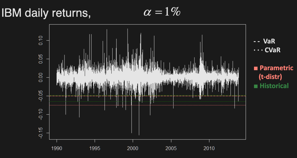
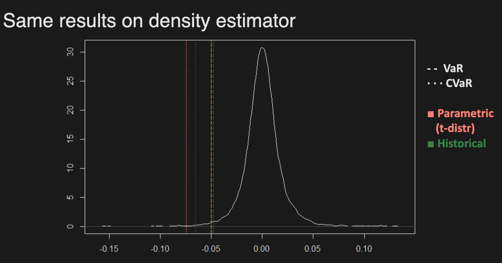
Historical simulation §

Instead of assuming a specific distribution, it uses the empirical distribution of returns estimated by historical data.

Monte Carlo simulation §

Even if returns are parametrically modelled, their resulting distribution is often intractable.

E.g. Consider a portfolio of 2 assets - one with normal returns, one with t-distributed returns. The distribution the portfolio return is not explicitly known.

We can simulate returns from such a model and treat simulated values as historical returns.

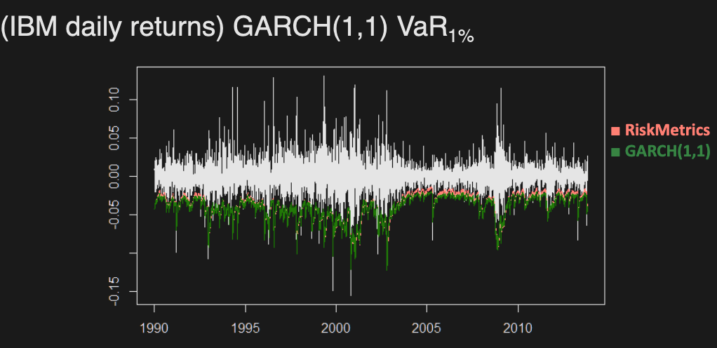
Time Series Models §

Static models assume independence over time (but allow dependence across assets)

RiskMetrics Model §

A simple time series model using the exponentially weighted moving average for return volatility

${\sigma }_t^2=\lambda {\sigma }_{t-1}^2+(1-\lambda )r_{t-1}^2$ where $r_t\sim N(0,{\sigma }_t^2)$

Typically, use $\lambda =.94$ for daily returns

GARCH(p, q) Model §

$r_t=\mu +{\sigma }_t{ϵ}_t$ where ${ϵ}_t$ are iid and ${\sigma }_t^2={\alpha }_0+{\sum }_{j=1}^p{\alpha }_j{r}_{t-j}^2+{\sum }_{k=1}^q{\beta }_k{\sigma }_{t-k}^2$

W7: Betting Strategies §

If we have a sequence of gambles where we have a positive expected payoff, how do we wager our bets for optimal results? We will look at a few different strategies below.

Setup. Consider a sequence of independent & identical gambles with

• Let p = P(win) $\in [0.5,1]$
• For each $1 placed, the payoff is $\{\begin{array}{ll}1& p\\ -1& q\end{array}$

Starting with initial wealth $V_0$, assume you bet a constant amount $X$ at each step. Find expected wealth $E(V_n)$ after n steps (ignoring ruin: $V_t\le 0$ for some $t>0$)

Define indicator RV of winning i-th bet: $I_i=\{\begin{array}{ll}1& p\\ 0& q\end{array}$

$$\begin{array}{rl}{V}_1& =V_0+X{I}_1-X(1-I_1)=V_0+X(2I_1-1)\\ V_2& =V_1+X{I}_2-X(1-I_2)=V_1+X(2I_2-1)=V_0+X(2(I_1+I_2)-2)\\ & ⋮\\ V_n& =V_0+X\left(2\underset{\sim Binomial(n,p)}{\underbrace{\sum _{i=1}^n{I}_i}}-n\right)\\ E(V_n)& =V_0+X\left(2E\left(\sum _{i=1}^n{I}_i\right)-n\right)\\ & =V_0+X(2np-n)\\ & =V_0+nX\underset{>0}{\underbrace{(2p-1)}}\end{array}$$

Notice that if $p<\frac{1}{2}$, $E(V_n)$ could be negative. Otherwise, we can expect to have some positive wealth at time n which increases linearly. The variance increases quadratically.

Assume we bet $1 at each step. Start with $V_0=M$. Find the probability of eventual ruin, i.e. $V_n=0$ for some n.

Let ${\pi }_i=P(\text{eventual ruin for }{V}_0=i),\forall i\ge 1$ and ${\pi }_0=1$

$${\pi }_i={\pi }_{i+1}\cdot p+{\pi }_{i-1}\cdot q,\forall i\ge 1$$

Assume solution of the form ${\pi }_i=y^i$

$$y^i=p{y}^{i+1}+q{y}^{i-1}\stackrel{i=1}{⟹}y=p{y}^2+q⟹p{y}^2-y+q=0$$

Solve quadratic:

$$\begin{array}{rl}y& =\frac{-b\pm \sqrt{b^2-4ac}}{2a}\\ & =\frac{-(-1)\pm \sqrt{(-1{)}^2-4pq}}{2p}\\ & =\frac{1\pm \sqrt{1-4p(1-p)}}{2p}\\ & =\frac{1\pm \sqrt{1-4p+4p^2}}{2p}\\ & =\frac{1\pm \sqrt{(2p-1{)}^2}}{2p}\\ & =\frac{1\pm (2p-1)}{2p}\\ & =\{\begin{array}{ll}1& \text{trivial sol’n}\\ \frac{1-2p+1}{2p}=1-\frac{p}{p}=\frac{q}{p}& \end{array}\end{array}$$

If $y=1$, then ${\pi }_i=y^i=1,\forall i\ge 0$. This is a trivial solution (probability of ruin = 1 at all times).

So $y=\frac{q}{p}$, and the probability of eventual ruin is ${\pi }_i=y^i=(\frac{q}{p}{)}^i,\forall i\ge 0$

Assume we bet everything (entire wealth) at each step. What is our expected wealth $E(V_n)$ after $n$ steps, not ignoring ruin?

$$\begin{array}{rl}{V}_n& =\{\begin{array}{ll}{V}_0\cdot 2^n& p^n\\ 0& 1-p^n\end{array}\\ E(V_n)& =2^n{V}_0\cdot p^n+0\cdot (1-p^n)=V_0(2p{)}^n\end{array}$$

Note that as $n\to \infty ,E(V_n)\to \infty$ since 2p>1. Wealth will grow exponentially.

Assume we bet a fixed fraction $f$ of wealth at each step. What is our expected wealth $E(V_n)$ after $n$ steps?

$$\begin{array}{rl}{V}_i& =\{\begin{array}{ll}{V}_{i-1}(1+f)& p\\ V_{i-1}(1-f)& q\end{array}\\ V_n& =V_{n-1}(1+f{)}^{I_n}(1-f{)}^{1-I_n}\\ & =V_0(1+f{)}^{{\sum }_{i=1}^n{I}_i}(1-f{)}^{n-{\sum }_{i=1}^n{I}_i}\\ E(V_n)& =E(V_0(1+f{)}^w(1-f{)}^{n-w})\leftarrow \text{w = |wins|}\\ & =V_0(1-f{)}^n\underset{{\left(q+p\frac{1+f}{1-f}\right)}^n}{\underbrace{E{\left(\frac{1+f}{1-f}\right)}^w}}\end{array}$$

This step uses the PGF (probabilistic generating function) of Binomial(n, p):

$$G_w(z)=E(z^w)=(q+pz{)}^n$$

Continuing:

$$\begin{array}{rl}E(V_n)& =V_0(1-f{)}^n{\left(q+p\frac{1+f}{1-f}\right)}^n\\ & =V_0(q(1-f))+p(1+f){)}^n\\ & =V_0(1-qf+pf{)}^n\\ & =V_0(1+f(p-\underset{1-p}{\underbrace{q}}){)}^n\\ & =V_0(1+f(\underset{>0}{\underbrace{2p-1}}){)}^n\end{array}$$

We have exponential growth and a low probability of ruin.

Kelly Criterion §

Bet fraction of wealth that maximizes expected log return (or equivalently log of $V_n$, or geometric average of returns).

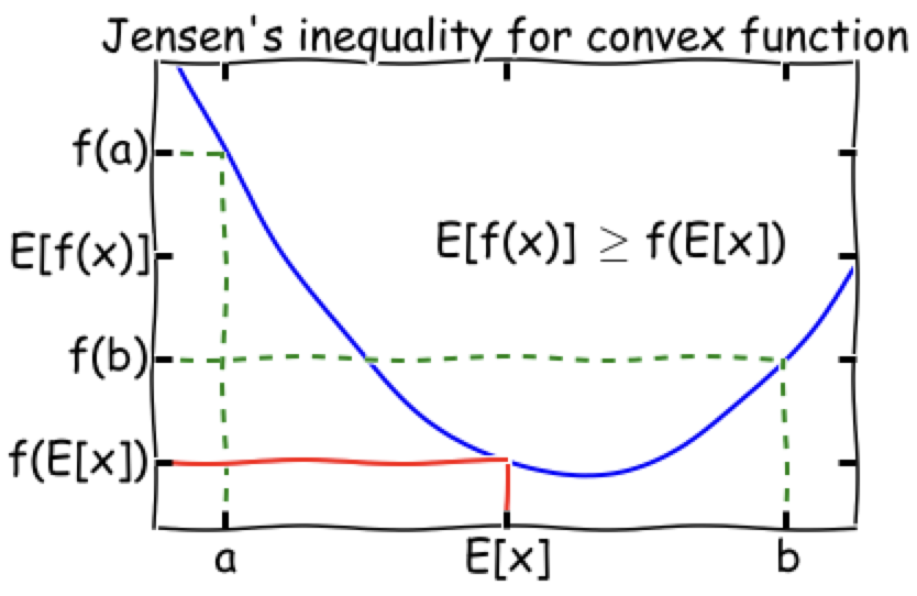
Note: by Jensen’s inequality, maximizing log wealth != maximizing wealth, i.e.

$$E(\log V_n)\ne \log (E(V_n))$$

What is the optimal value of the fraction? §

$$\begin{array}{rl}E\left(\log \frac{V_n}{V_0}\right)& =E\left(\log \left(\frac{\cancel{V_0}(1+f{)}^w(1-f{)}^{n-w}}{\cancel{V_0}}\right)\right)\\ & =E(w\log (1+f)+(n-w)\log (1-f))\\ & =\log (1+f)E(w)+\log (1-f)(n-E(w))\\ & =\log (1+f)np+\log (1-f)(n-np)\\ & =\log (1+f)np+\log (1-f)nq\\ & =G(f)\end{array}$$

Now maximize G(f) w.r.t. $f$ and set to 0

$$\begin{array}{rl}\frac{dG(f)}{df}& =\frac{d}{df}(\log (1+f)np+\log (1-f)nq)\\ 0& =n\left(\frac{1}{1+f}p-\frac{1}{1-f}q\right)\\ \frac{p}{1+f}& =\frac{q}{1-f}\\ p(1-f)& =q(1+f)\\ p-q& =f(p+q)\\ f^{\ast }& =p-q=2p-1\end{array}$$

The optimal fraction is the difference between P(win) and P(lose).

What is the geometric average of the returns as $n\to \infty$? §

Denoting the growth rate from $i-1$ to $i$ with $r_i=\frac{V_i}{V_{i-1}}$, the geometric average is

$$\begin{array}{rl}\sqrt[n]{r_1\times \cdots \times r_n}& ={\left[\prod _{i=1}^n(1+f{)}^{I_i}(1-f{)}^{1-I_i}\right]}^{1/n}\\ & =(1+f{)}^{{\sum }_{i=1}^n{I}_i/n}(1-f{)}^{{\sum }_{i=1}^n(1-I_i)/n}\\ & =(1+f{)}^{W_n/n}(1-f{)}^{1-W_n/n}\end{array}$$

where $W_n\sim Binom(n,p)$

By SLLN, $\frac{W_n}{n}\to p$ as $n\to \infty$, so the geometric average $\to (1+f{)}^p(1-f{)}^q$

General Setup §

Now consider a general sequence of bets, where $1 bet +$a if win and −$b if lose. (In previous examples, a = b = 1, and the bet is favourable, i.e.$pa>qb$.)

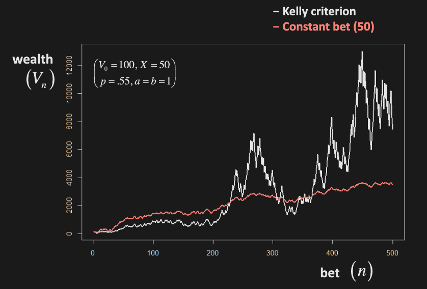
The Kelly criterion optimal fraction to bet is: (Proved in PS 7.1b)

$$f^{\ast }=\frac{pa-qb}{ab}$$

In the following example, f = 0.55 - 0.45 = 0.1

Investing Example §

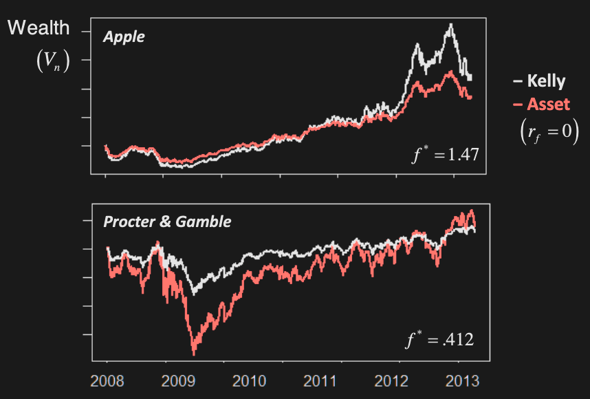
Now consider the following. We have a…

• risk free asset with return $r_f$
• risky asset with return $R$: $E(R)=\mu ,\mathbb{V}(R)={\sigma }^2$

We invest fraction f of wealth into risky asset & remaining (1–f) into risk-free asset.

Apply Kelly Criterion to find f that maximizes logarithm of wealth:

$$\begin{array}{rl}{V}_1& =f{V}_0\cdot (1+R)+(1-f)V_0\cdot (1+r_f)\\ & =V_0[\cancel{f}+fR+1\cancel{-f}+r_f-f{r}_f]\\ & =V_0[1+r_f+f(R-r_f)]\\ \log \left(\frac{V_n}{V_0}\right)& =\log \left(\prod _{t=1}^n\frac{V_t}{V_{t-1}}\right)=\sum _{t=1}^n\log (1+r_f+f(R_t-r_f))\\ E\left[\log \left(\frac{V_n}{V_0}\right)\right]& =\sum _{t=1}^{n}E[\log (1+r_f+f\cdot (R_t-r_f))]\\ & =nE[\log (1+r_f+f\cdot (R_t-r_f))]\end{array}$$

Use Taylor expansion for $x_0=\log (1+r_f+f(R_t-r_f))$ around $1+r_f$

$g^{\prime }(x_0+\delta )\approx g(x_0)+g^{\prime }(x_0)\delta +\frac{1}{2}{g}^{\prime \prime }(x_0){\delta }^2$

Applying this, we get

$$\begin{array}{rl}\log (\underset{x_0}{\underbrace{1+r_f}}+\underset{\delta }{\underbrace{f\cdot (R_t-r_f)}})& \approx \underset{g(x_0)}{\underbrace{\log (1+r_f)}}+\underset{g^{\prime }(x_0)}{\underbrace{\frac{1}{1+r_f}}}f\cdot (R_t-r_f)+\frac{1}{2}\underset{g^{\prime \prime }(x_0)}{\underbrace{\left(-\frac{1}{(1+r_f{)}^2}\right)}}{f}^2\cdot (R_t-r_f{)}^2\\ E(\log (1+r_f+f\cdot (R_t-r_f)))& \approx \log (1+r_f)+\frac{1}{1+r_f}f\cdot \underset{\mu -r_f}{\underbrace{E(R_t-r_f)}}+\frac{1}{2}\left(-\frac{1}{(1+r_f{)}^2}\right)f^2\cdot \underset{({\sigma }^2+{\mu }^2)+r_f^2-2\mu r_f}{\underbrace{E[(R_t-r_f{)}^2]}}\\ & \approx \log \left(1+r_f\right)+f\frac{\left(\mu -r_f\right)}{\left(1+r_f\right)}-f^2\frac{{\sigma }^2+{\left(\mu -r_f\right)}^2}{2{\left(1+r_f\right)}^2}\\ & =G(f)\end{array}$$

Differentiate w.r.t. f and set to 0:

$$\begin{array}{rl}& \\ \frac{\partial }{\partial f}G(f)& =0\\ \frac{\mu -r_f}{1+r_f}-f\frac{{\sigma }^2+(\mu -r_f{)}^2}{(1+r_f{)}^2}& =0\\ f^{\ast }& =\left(1+r_f\right)\frac{\left(\mu -r_f\right)}{{\sigma }^2+(\mu -r_f{)}^2}\end{array}$$

Since ${\sigma }^2\gg \mu -r_f$, we have

$$f^{\ast }\approx \left(1+r_f\right)\frac{\left(\mu -r_f\right)}{{\sigma }^2}$$

Theoretical properties §

In the long term ($n\to \infty$) with probability 1, a strategy based on Kelly criterion:

1. Maximizes limiting exponential growth rate of wealth
2. Maximizes median of final wealth
   • Half of distribution is above median & half below it
3. Minimizes the expected time required to reach a specified goal for the wealth

Criticism §

• Can have considerable wealth volatility (b/c of multiplicative bet amounts)
• Does not account for the uncertainty in probability of winning
  • Many practitioners use fractional or partial Kelly, i.e. using smaller than Kelly fraction (e.g., f*/2)
• In practice, investing horizons are not infinite and there are many other considerations (e.g. transaction costs, short-selling limits etc)

W8: Statistical Arbitrage §

Statistical Arbitrage (StatArb) refers to trading strategies that utilize the “statistical mispricing” of related assets

StatArb strategies are typically short term and market neutral, involving long & short positions simultaneously

Examples of StatArb strategies:

• Pairs trading
• Index Arbitrage
• Volatility Arbitrage
• Algorithmic & High Frequency Trading

Pairs Trading §

• Original & most well-known StatArb technique developed by Morgan Stanley quants
• Profit not affected by overall market movement (market neutral)
• Contrarian strategy profits from price convergence of related assets

Main idea §

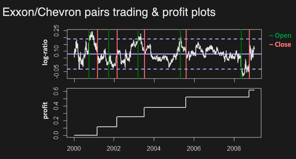
1. Select pair of assets “moving together”, based on certain criteria
2. If prices diverge beyond certain threshold, buy low sell high
3. If prices converge again, reverse position and profit

Example §

Let $L$ = price of lower asset, $H$ = price of higher asset.

• Open the position when prices diverge: buy $1 of low asset ($\frac{1}{L_0}$ units), sell $1 of high asset ($\frac{1}{H_0}$ units)
  • cost = $\frac{1}{L_0}{L}_0-\frac{1}{H_0}{H}_0=0$
• Close the position when prices converge
  • profit = $\frac{1}{L_0}{L}_c-\frac{1}{H_0}{H}_c$ (c stands for closing)

Profitability is determined by asset price ratios (hence the use of log ratios for modelling):

$$\begin{array}{rl}\frac{H_c}{H_0}-\frac{L_c}{L_0}& <or>0\\ \frac{H_c}{H_0}& <or>\frac{L_c}{L_0}\\ \log \left(\frac{H_c}{L_c}\right)& <or>\log \left(\frac{H_0}{L_0}\right)\end{array}$$

The strategy is market neutral, i.e. profitability is not affected by market movement - Assets typically have common market betas

What can go wrong? §

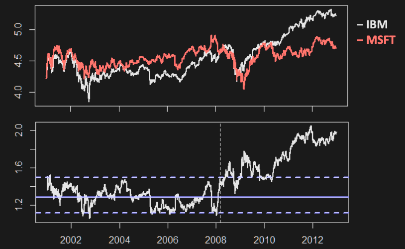
Prices may not converge.

Factors to consider §

1. Which pairs to trade
2. When to open trade
3. What amounts to buy/sell
4. When to close trade
5. When to bail out of trade

Most of these decisions involve trade-offs, so how do we select pairs to trade?

• Profitable pairs must have log-ratio with strong mean reversion
  • Note: Mean reversion is not the same as simply having constant mean

Mean Reversion §

Suggests log-ratio process $\left\{X_t\right\}$ is stationary

• $E(X_t)=\mu ,\forall t$

• $Var(X_t)={\sigma }^2<\infty ,\forall t$

• $Cov(X_t,X_s)=Cov(X_{t+r},X_{s+r}),\forall r,s,t$

• Autocorrelation function $\rho (h),\forall h=0,1,\dots$ describes linear dependence at lag $h=|t-s|$

Stationarity ensures process will revert back to its mean within reasonable time.

E.g. Let $X_t=\log (\frac{H_t}{L_t}){\sim }^{iid}N(0,{\sigma }^2),\forall t=1,2,\dots$

If $X_0=2\sigma$, what is the expected time until $X_T\le 0$? I.e. until $\log H_t-\log L_t<0$

On any day t, $P(X_t\le 0)=\frac{1}{2}$

Let T = # days until $\{X_t\le 0\}$ for the first time. T is called hitting time, it is equal to # trials until 1st success (if $X\le 0$), so $T\sim Geom(p=\frac{1}{2})$ which has prob mass function

$$p_T(t)={\left(\frac{1}{2}\right)}^t,\forall t\ge 1$$

The expected time is hence

$$E(T)=\frac{1}{p}=2$$

E.g. Let $X_t=\log (\frac{P{1}_t}{P{2}_t})\sim$ Brownian Motion (BM) (continuous time Random Walk)

For any $X_0=c>0$, show that the expected time until $X_T\le 0$ is infinite.

Let $T_c$ = {first time standard BM with $W_0=0$} hits level c Let $M_t=\max \left\{W_u;0\le u\le t\right\}⟹M_t\sim |W_t|$

This means:

$$\begin{array}{r}P(T_c\le t)=P(M_t\ge c)=P(|W_t|\ge c)=2\Phi \left(-\frac{c}{\sqrt{t}}\right)\end{array}$$

PDF of $T_c$ is given by $f(t)=\frac{d}{dt}P(T_c\le t)$

$$\begin{array}{rl}f(t)& =\frac{d}{dt}\left[2\Phi \left(-\frac{c}{\sqrt{t}}\right)\right]\\ & =2\varphi \left(-\frac{c}{\sqrt{t}}\right)\cdot \frac{d}{dt}\left(-\frac{c}{\sqrt{t}}\right)\\ & =2\varphi \left(-\frac{c}{\sqrt{t}}\right)\cdot \left(\frac{1}{2}\frac{c}{\sqrt{t^3}}\right)\\ & =\frac{1}{\sqrt{2\pi }}{e}^{-\frac{1}{2}\frac{c^2}{t}}\frac{c}{\sqrt{t^3}}\\ E(T_c)& ={\int }_0^{\infty }t\cdot f(t)dt={\int }_0^{\infty }t\cdot \frac{c}{\sqrt{2\pi t^3}}{e}^{-\frac{c^2}{2t}}dt\\ & =\frac{c}{\sqrt{2\pi }}{\int }_0^{\infty }\frac{1}{\sqrt{t}}{e}^{-c^2/2t}dt\\ & \ge \frac{c^{\prime }}{\sqrt{2\pi }}{\int }_0^a\frac{1}{\sqrt{t}}dt+{\int }_a^{\infty }\frac{1}{\sqrt{t}}{e}^{-c^2/2t}dt\to \infty \\ ⟹E(T_c)& =\infty \end{array}$$

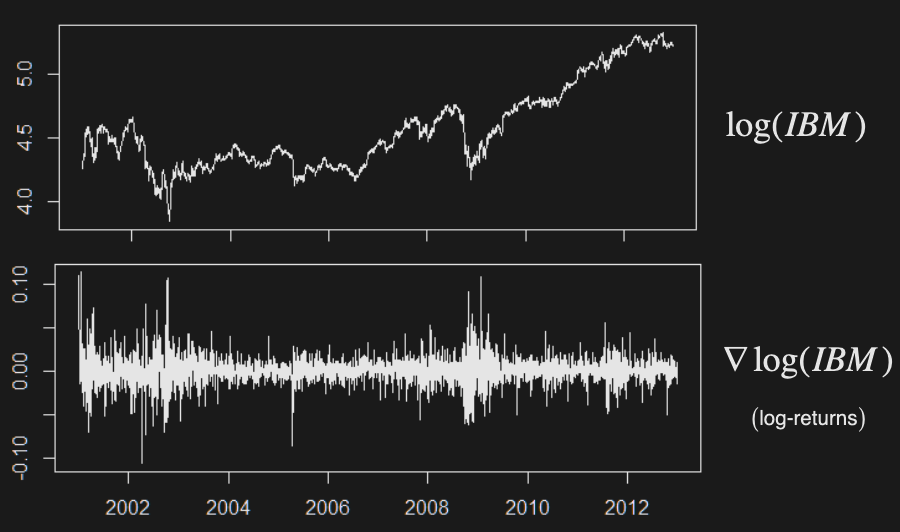
Integrated Series §

A non-stationary time series $\left\{X_t\right\}$ whose difference $\left\{\nabla X_t=X_t-X_{t-1}\right\}$ is stationary

Asset log prices are not stationary - will need to apply differencing

Although $r_t=\log (\frac{S_t}{S_{t-1}})$ follows a stationary process, $\log S_t=\log S_0+{\sum }_{i=1}^t{r}_i$ is a random walk

Example: IBM stock price before and after differencing

Cointegration §

Two integrated series $\left\{X_t,Y_t\right\}$ are cointegrated if there exists a linear combination of them that is stationary.

Consider a vector of time series $x_t$. If each element becomes stationary after differencing, but a linear combination ${\alpha }^{\prime }{x}_t$ is already stationary, then $x_t$ is said to be co-integrated with $\alpha$, which is the co-integrating vector.

There may be several such co-integrating vectors so that $\alpha$ becomes a matrix. Interpreting ${\alpha }^{\prime }{x}_t=0$ as a long run equilibrium, co-integration implies that deviations from equilibrium are stationary, with finite variance, even though the series themselves are non-stationary and have infinite variance.

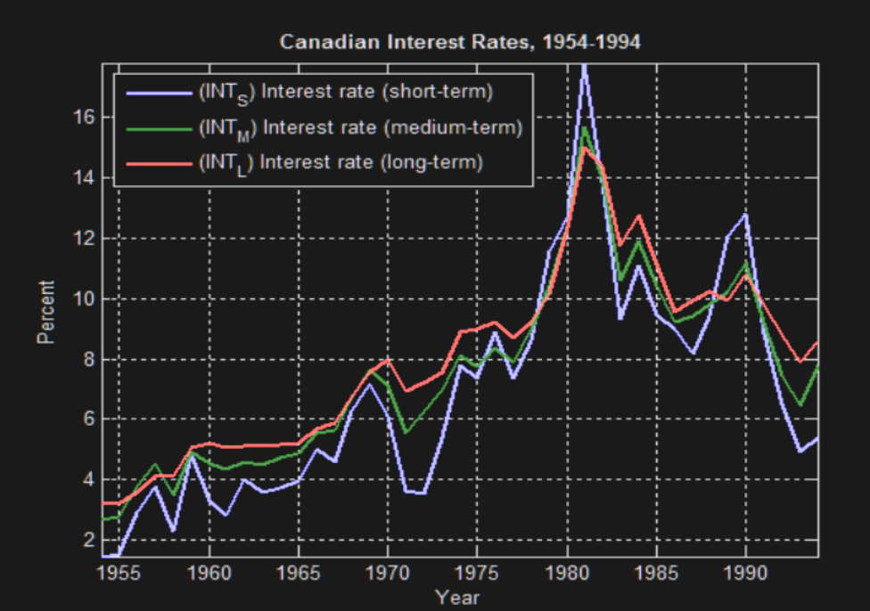
For pairs trading, we want to find assets which are cointegrated (their log difference is mean reverting, and thus stationary)

E.g. ST, MT, and LT interest rates are co-integrated - they move together but behave as random walks individually

E.g. Let $\left\{W_t\right\}$ be random walk, and $\{\begin{array}{c}{X}_t=W_t+{\epsilon }_t\\ Y_t=W_t+{\eta }_t\end{array}$ where ${\epsilon }_t,{\eta }_t{\sim }^{\text{iid }}N\left(0,{\sigma }^2\right)$

Show that $\left\{X_t,Y_t\right\}$ are cointegrated

First, we need to show $X_t,Y_t$ are integrated (not stationary, with stationary 1st order differences).

$$\mathbb{V}\left(X_t\right)=\mathbb{V}\left[W_t+{ϵ}_t\right]=\mathbb{V}\left(W_t\right)+\mathbb{V}\left({ϵ}_t\right)=t{\sigma }_w^2+{\sigma }^2⟹\text{ not stationary }$$

Which is the same case for $Y_t$

Next, show cointegration by showing $X_t-X_{t-1}$ is stationary.

$$\begin{array}{rl}\nabla X_t=X_t-X_{t-1}& =W_t+{ϵ}_t-W_{t-1}-{ϵ}_{t-1}=\underset{{\nu }_t\sim WN(0,{\sigma }^2)}{\underbrace{\left(W_t-W_{t-1}\right)}}+{ϵ}_t-{ϵ}_{t-1}\\ E(\nabla X_t)& =E({\nu }_t)+E({ϵ}_t)-E({ϵ}_{t-1})=0⟹\text{not stationary}\\ V(\nabla X_t)& =V({\nu }_t)+V({ϵ}_t)+V({ϵ}_{t-1})={\sigma }^2+2{\sigma }_{ϵ}^2\\ Cov(\nabla X_t,\nabla X_s)& =\gamma (t-s)\end{array}$$

If |t-s| > 1, $Cov(\nabla X_t,\nabla X_s)=Cov({\nu }_t+{ϵ}_t-{ϵ}_{t-1},{\nu }_s+{ϵ}_s-{ϵ}_{s-1})=0$

If |t-s| = 1, $Cov(\nabla X_t,\nabla X_s)=Cov({\nu }_t+{ϵ}_t-{ϵ}_{t-1},{\nu }_{t+1}+{ϵ}_{t+1}-{ϵ}_t)=Cov({ϵ}_t,-{ϵ}_t)=-{\sigma }_{ϵ}^2$

$\nabla X_t$ is thus stationary $⟹X_t\sim I(1)$ is integrated of order 1 (and similarly for $Y_t$)

$X_t-Y_t=w_t+{ϵ}_t-(w_t+n_t)={ϵ}_t-n_t\stackrel{iid}{\sim }N(0,{\sigma }_{ϵ}^2+{\sigma }_n^2)$ is stationary, so $(X_t,Y_t)$ are cointegrated.

Stationarity Tests §

Hypothesis test for $\{\begin{array}{l}{H}_0\text{ : series is integrated }\\ H_1\text{ : series is stationary }\end{array}$

Idea: fit $X_t=\beta X_{t-1}+{\epsilon }_t$ to data and test $\{\begin{array}{l}{H}_0:\beta =1\\ H_1:\beta <1\end{array}$

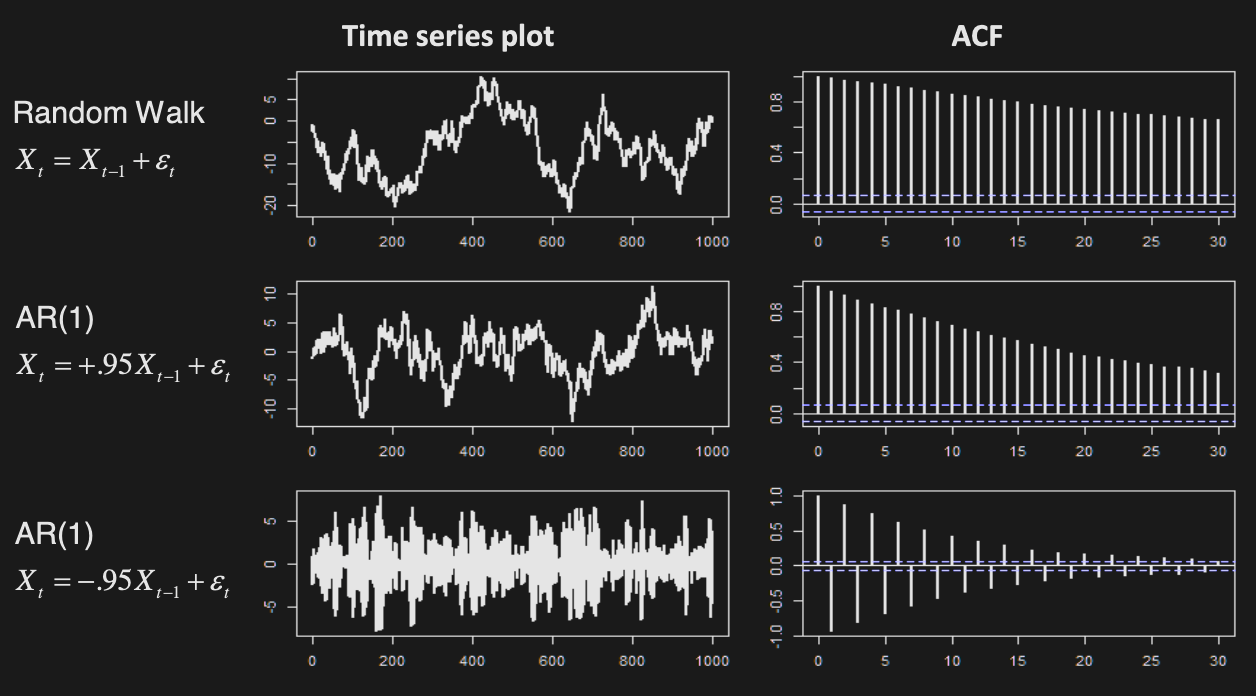
For random walk, we fail to reject the null hypothesis that $X_t$ is integrated.

Issue: we don’t know which linear combination to check for stationarity

Two-step method §

• Estimate linear relationship between variables

• Test resulting difference series (residuals) for stationarity

• Example: regress Chevron on Exxon log-prices

  • 
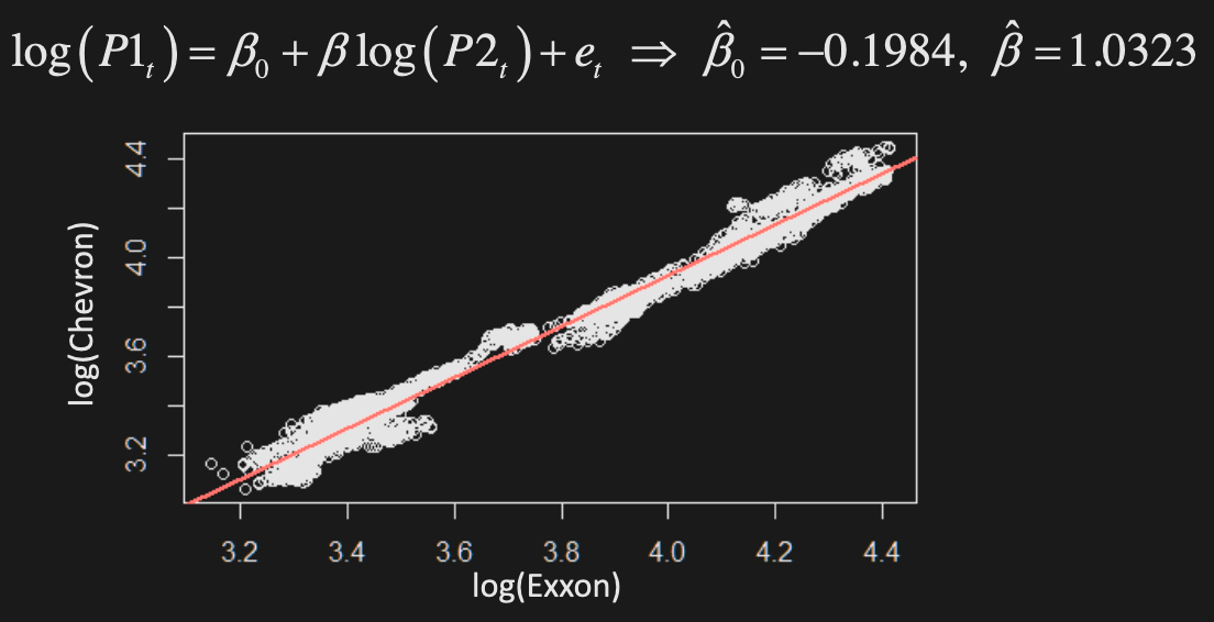
  • Then, test residuals for stationarity: reject the null hypothesis that it is integrated -

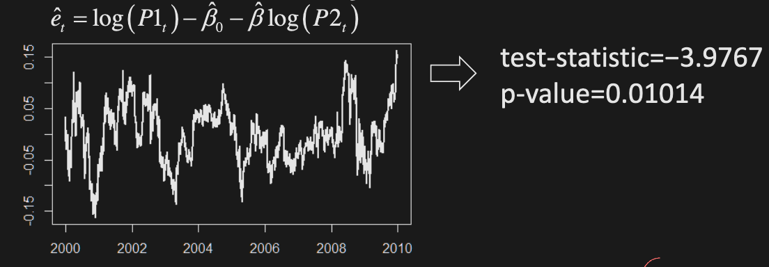
• Problems:

  • Regressing P1 and P2 can give different results than regressing the other way around.
  • There is estimation error for residuals.

• Can be used to address spurious regression

  • Results of random walk (integrated series) regressions are NOT reliable
    • Consider 2 independent random walks $\left\{W_t,V_t\right\}$
    • When you regress $W_t={\beta }_0+\beta V_t+e_t,t=1,\dots ,n$ you are NOT guaranteed that $\hat{\beta }\to 0$ as the sample size $n\to \infty$ (i.e. not consistent)

Vector Error Correction models (VECM) §

Combined treatment of dynamics & cointegration, using Vector AutoRegressive (VAR) models

Index Arbitrage §

• Indices measure value/performance of financial markets
  • Dow-Jones Industrial Average (DJIA): Simple average of 30 major US stock prices (since 1896)
  • Standard & Poor (S&P) 500: Weighted (cap-base) average of 500 large NYSE & NASDAQ listed companies
• Financial indices are NOT traded instruments. However, there are many financial products whose value is directly related to indices:
  • Mutual funds: e.g., Vanguard® 500 Index Fund
  • Exchange-Traded-Funds (ETF’s): e.g., SPDR or iShares S&P500 Index
  • Futures: e.g., E-Mini S&P futures
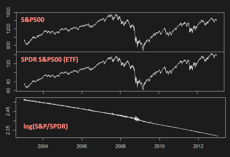
• Financial products based on indices essentially offer a sophisticated version of multivariate cointegration
  • For an index of N assets ${\left\{S_i\right\}}_{i=1}^N$ w/ weights ${\left\{w_i\right\}}_{i=1}^N$, the index level is $I(t)={\sum }_{i=1}^N{w}_i\times S_i(t)$
  • It has a co-integrating relationship with $F(t)$, an instrument tracking index (e.g. futures)

$$F(t)-I(t)=F(t)-\sum _{i=1}^N{w}_i\times S_i(t)\sim \text{ stationary }$$

Volatility Arbitrage §

• VolArb is implemented with derivatives, primarily options
• The higher the volatility, the higher the option price

Consider European options:

• For Black-Scholes formula, the only unobserved input is volatility $\sigma$, which has to be estimated

• Implied volatility ${\sigma }_i$i s the input that makes Black-Scholes price equal to observed market price

  • not estimated from underlying asset dynamics

• If volatility will increase in the future, beyond what current options prices warrant (implied vol), some possible strategies are:

  • straddles (long at the money call and put)
  • strangles (long out of the money call and put)
  • delta-hedged long call or put

• Delta-neutral strategies eliminate effects of asset movement

  • 

• Common approach is to describe the evolution of volatility with GARCH (Generalized AutoRegressive Conditional Heteroskedasticity) models

$$\begin{array}{c}{y}_t={\sigma }_t\cdot {\epsilon }_t,{\epsilon }_t{\sim }^{iid}N(0,1)\\ {\sigma }_t^2={\alpha }_0+\sum _{j=1}^p{\alpha }_j{y}_{t-j}^2+\sum _{k=1}^q{\beta }_k{\sigma }_{t-k}^2\end{array}$$

W9: Monte Carlo Simulation §

Numerical Option Pricing §

3 basic numerical option pricing methods:

1. Binomial trees
2. Finite difference (based on Black Scholes PDE)
3. Monte Carlo simulation (based on SDE for asset prices & risk neutral valuation)

Multivariate Normal Properties §

If $\mathbf{X}=\left[\begin{array}{l}{\mathbf{X}}_1\\ {\mathbf{X}}_2\end{array}\right]\sim N\left(\mathbf{\mu }=\left[\begin{array}{l}{\mathbf{\mu }}_1\\ {\mathbf{\mu }}_2\end{array}\right],\mathbf{\Sigma }=\left[\begin{array}{cc}{\mathbf{\Sigma }}_{11}& {\mathbf{\Sigma }}_{12}\\ {\mathbf{\Sigma }}_{21}& {\mathbf{\Sigma }}_{22}\end{array}\right]\right)$, then:

Marginals §

$${\mathbf{X}}_1\sim \mathrm{N}\left({\mathbf{\mu }}_1,{\mathbf{\Sigma }}_{11}\right)$$

Linear combinations §

$$\mathbf{a}+{\mathbf{B}}^{\top }\mathbf{X}\sim \mathbf{N}\left(\mathbf{a}+{\mathbf{B}}^{\top }\mathbf{\mu },{\mathbf{B}}^{\top }\mathbf{\Sigma }\mathbf{B}\right)$$

Conditionals §

$${\mathbf{X}}_1\mid \left({\mathbf{X}}_2=\mathbf{x}\right)\sim \mathbf{N}\left({\mathbf{\mu }}_1+{\mathbf{\Sigma }}_{12}{\mathbf{\Sigma }}_{22}^{-1}\left(\mathbf{x}-{\mathbf{\mu }}_2\right),{\mathbf{\Sigma }}_{11}-{\mathbf{\Sigma }}_{12}{\mathbf{\Sigma }}_{22}^{-1}{\mathbf{\Sigma }}_{21}\right)$$

Notice how ${\mathbf{\Sigma }}_{12}=0⟺{\mathbf{X}}_1|({\mathbf{X}}_2=x)\sim N({\mathbf{\mu }}_1,{\mathbf{\Sigma }}_{11})$

Brownian Motion §

$W_T\sim N(0,T)$ forms the building block of continuous stochastic models

Recall Ito Processes from STAC70:

A (one-dimensional) Itô process is a stochastic process ${\left\{X_t\right\}}_{t\ge 0}$ of the form

$$X_t=x_0+{\int }_0^t{a}_{s}ds+{\int }_0^t{b}_{s}d{B}_s$$

where ${\left\{a_t\right\}}_{t\ge 0}$ and ${\left\{b_t\right\}}_{t\ge 0}$ are adapted processes such that the integrals are defined. Equivalently, we can write this as

$$d{X}_t=a_{t}dt+b_{t}d{B}_t$$

The Brownian motion ${\left\{B_t\right\}}_{t\ge 0}$ is an Itô process. (Pick $a_t\equiv 0$ and $b_t\equiv 1$.)

The general Brownian motion with (constant) drift $\mu \in \mathbb{R}$ (and constant volatility $\sigma >0$) is an Itô process. (Pick $a_t\equiv \mu$ and $b_t\equiv \sigma$.)

$$X_t=x_0+\mu t+\sigma B_t$$

Standard Brownian Motion §

$\left\{W_t\right\}$ with the following properties:

• $W_0=0$
• $(W_t-W_s)|W_s\sim N(0,t-s)$

Arithmetic Brownian Motion §

$\left\{X_t\right\}$ with drift $\mu$ and volatility $\sigma$ and the following properties:

• $X_0=0$
• $(X_t-X_s)|X_s\sim N(\mu (t-s),{\sigma }^2(t-s))$

$⟹X_t|X_s=x\sim N(x+\mu (t-s),{\sigma }^2(t-s))$

SDE form:

$$\begin{array}{rl}{X}_t-X_0& ={\int }_0^t\mu ds+{\int }_0^t\sigma d{W}_s\\ & =\mu t+\sigma (W_t-W_0)\\ d{X}_t& =\mu dt+\sigma d{W}_t\end{array}$$

E.g. For $d{X}_t=\mu dt+\sigma d{W}_t$, find distribution of $X_t|X_s=x$

For $s<t$

$$\begin{array}{rl}\left[\begin{array}{c}{X}_s\\ X_t\end{array}\right]& \sim N(\mu \left[\begin{array}{c}s\\ t\end{array}\right],{\sigma }^2\left[\begin{array}{cc}s& s\\ s& t\end{array}\right])\\ ⟹\left[\begin{array}{c}{X}_t\\ X_s\end{array}\right]& \sim N(\mu \left[\begin{array}{c}t\\ s\end{array}\right],{\sigma }^2\left[\begin{array}{cc}t& s\\ s& s\end{array}\right])\\ ⟹X_t|X_s=x& \sim N\left(\mu t+{\sigma }^{2}s\frac{1}{{\sigma }^{2}s}(x-\mu s),{\sigma }^2\left(t-s\frac{1}{s}s\right)\right)\\ & \sim N(x+\mu (t-s),{\sigma }^2(t-s))\end{array}$$

$$\begin{array}{rl}Cov(W_s,W_t)& =Cov(W_s,W_s+(W_t-W_s))\\ & =Cov(W_s,W_s)+\cancel{Cov(W_s,(W_t-W_s)})\\ & =Var(W_s)\\ & =s\end{array}$$

For $s\in (0,t)$ (Brownian Bridge)

$$\begin{array}{rl}\left[\begin{array}{c}{X}_s\\ X_t\end{array}\right]& \sim N(\mu \left[\begin{array}{c}s\\ t\end{array}\right],{\sigma }^2\left[\begin{array}{cc}s& s\\ s& t\end{array}\right])\\ X_s|X_t=x& \sim N\left(\mu s+s\frac{1}{t}(x-\mu t),{\sigma }^2\left(s-s\frac{1}{t}s\right)\right)\\ & \sim N\left(\frac{s}{t}x,{\sigma }^2\frac{s(t-s)}{t}\right)\end{array}$$

Geometric Brownian Motion §

Process $\left\{S_t\right\}$ whose logarithm follows ABM

$$\begin{array}{rl}{S}_t& =S_0{e}^{\log \left(\frac{S_t}{S_0}\right)}\text{where }\log \left(\frac{S_t}{S_0}\right)\sim N(\mu t,{\sigma }^{2}t)\\ & \sim S_0\log N(\mu t,{\sigma }^{2}t)\end{array}$$

SDE form:

$$\begin{array}{rl}d\log (S_t)& =\mu dt+\sigma d{W}_t\\ d{S}_t& =\left(\mu +\frac{{\sigma }^2}{2}\right)S_{t}dt+\sigma S_{t}d{W}_t\end{array}$$

Risk Neutral Pricing §

A risk-neutral (RN) measure or equivalent martingale measure (EMM) is a probability measure under which discounted asset prices are martingales.

Martingale: a stochastic process with the property $E(X_{n+1}|X_1,...,X_n)=X_n$

Assuming GBM for asset $\left\{S_t\right\}$ and risk-free interest rate $r$, there exists a probability measure such that

$$\begin{array}{rl}d{S}_t& =r{S}_{t}dt+\sigma S_{t}d{W}_t\\ S_t& \sim S_0\times \log N\left(\left(r-\frac{{\sigma }^2}{2}\right)t,{\sigma }^{2}t\right)\end{array}$$

The arbitrage-free price of any European derivative with payoff $G_T=f\left(S_T\right)$ is given by discounted expectation w.r.t. RN measure

$$G_0=\mathbb{E}\left[e^{-rT}{G}_T\right]=\mathbb{E}\left[e^{-rT}f\left(S_T\right)\right]$$

E.g. Show that under RN measure, $E(S_t)=S_0{e}^{rt}$. More generally, $E(S_t/e^{rt}|S_s)=S_s/e^{rt}$.

$$\begin{array}{r}E(S_t)=E(S_0{e}^{\log (S_t/S_0)})=S_0\mathbb{E}(e^Y)\text{where }Y=\log \left(\frac{S_t}{S_0}\right)\sim N\left(\left(r-\frac{{\sigma }^2}{2}\right)t,{\sigma }^{2}t\right)\end{array}$$

Use the Normal MGF:

If $X\sim N(\mu ,{\sigma }^2)$, then $m_X(z)=e^{\mu z+\frac{1}{2}{\sigma }^2{z}^2}$

$$m_Y(1)=\exp \left\{\underset{E(Y)}{\underbrace{\left(r-\frac{{\sigma }^2}{2}\right)t}}+\frac{1}{2}\underset{\mathbb{V}(Y)}{\underbrace{{\sigma }^{2}t}}\right\}=S_0{e}^{rt}$$

E.g. Find price of forward contract $F_{0,T}$ (no dividends)

$$G_T=f(S_T)=(S_T-F_{0,T})$$

We know $G_0=0$ (forward contracts involve no cashflow at t=0)

By risk neutral pricing, $G_0=E(e^{-rT}{G}_T)$

$$\begin{array}{rl}0& =\mathbb{E}(e^{-rT}(S_T-F_{0,T}))\\ 0& =\mathbb{E}(S_T)-F_{0,T}\\ F_{0,T}& =\mathbb{E}(S_T)=e^{rT}\mathbb{E}(\underset{\sim mgle}{\underbrace{e^{-rT}{S}_T}})=e^{rT}{S}_0\end{array}$$

Estimating Expectations §

If $\mathbb{E}\left[e^{-rT}f\left(S_T\right)\right]$ cannot be calculated exactly, it can be estimated/approximated by simulation:

• Generate N independent random variates $S_i(T),i=1,\dots ,N$ based on RN measure (i = iterations, not time)
• By Law of Large Numbers (SLLN)

$${\hat{G}}_0=\frac{1}{n}\sum _{i=1}^n{e}^{-rT}f\left(S_i(T)\right)\to \mathbb{E}\left[e^{-rT}f\left(S_T\right)\right]\text{, with prob. }1$$

• Moreover, by Central Limit Theorem (CLT)

$$\frac{{\hat{G}}_0-G_0}{s_G/\sqrt{n}}{\sim }^{appr.}N(0,1)\text{, where }{s}_G^2=\frac{1}{n-1}\sum _{i=1}^n{\left[e^{-rT}f\left(S_i(T)\right)-{\hat{G}}_0\right]}^2$$

E.g. Show estimator of $\mathbb{E}(e^{-rT}f(S_T))$ is consistent, and build 95% confidence interval for $G_0$

Estimator: $\mathbb{E}[e^{-rT}f(S_T)]$

Build a 95% confidence interval for $G_0$ as well

$$\begin{array}{rl}\mathbb{E}(\widehat{G_0})& =\mathbb{E}\left[\frac{1}{n}\sum _{i=1}^n{e}^{-rT}f(S_i(T))\right]\\ & =\frac{1}{n}\sum _{i=1}^n\underset{G_0}{\underbrace{\mathbb{E}[e^{-rT}f(S_i(T))]}}=\frac{1}{n}n{G}_0=G_0\end{array}$$

Confidence interval:

$$\widehat{G_0}\pm 1.96\times \frac{S_G}{\sqrt{n}}$$

European Call §

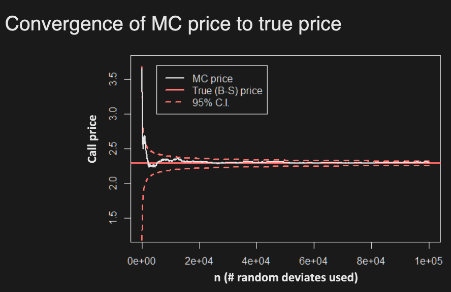
Estimate European call price w/ simulation

• Asset price dynamics: $d{S}_t=r{S}_{t}dt+\sigma S_{t}d{W}_t$
• Payoff function for strike K & maturity T: $f(S_T)=(S_T-K{)}_T$

Generate random asset price variates as:

$$S_i(T)=S(0)\exp \left\{\left(r-\frac{{\sigma }^2}{2}\right)T+\sigma \sqrt{T}{Z}_i\right\}$$

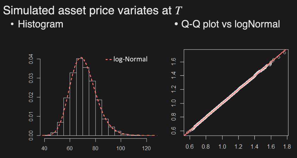
where $Z_i$ is standard Normal variate

Multiple assets §

Payoff of some options depends on prices of multiple assets

E.g. exchange (outperformance) option w/ payoff

$$\max \left\{S_1(T)-S_2(T),0\right\}=(S_1(T)-S_2(T){)}_{+}$$

Monte Carlo option pricing requires simulating and averaging multiple asset prices/paths. We cannot simply simulate each asset separately since there could be cross-asset dependence.

Multivariate Brownian Motion §

Define $d$-dimensional standard BM

$$\mathbf{W}(t)=\left[\begin{array}{c}{W}_1(t)\\ ⋮\\ W_d(t)\end{array}\right]\text{ with correlation matrix }\mathbf{\rho }=\left[\begin{array}{ccc}1& \dots & {\rho }_{1d}\\ ⋮& \ddots & ⋮\\ {\rho }_{d1}& \cdots & 1\end{array}\right]$$

to have independent Normal increments

$$\mathbf{W}(t)-\mathbf{W}(s)\mid \mathbf{W}(s)\sim N_d(0,(t-s)\mathbf{\rho })$$

Note: increments are independent over time, but can be dependent across dimensions!

Multivariate ABM §

$\{\mathbf{X}(t)\}$ w/ SDE $d\mathbf{X}(t)=\mu dt+\mathbf{\sigma }d\mathbf{W}(t)$, where

$$\mathbf{\mu }={\left[\begin{array}{lll}{\mu }_1& \cdots & {\mu }_d\end{array}\right]}^{\top },\mathbf{\sigma }={\left[\begin{array}{lll}{\sigma }_1& \cdots & {\sigma }_d\end{array}\right]}^{\top }$$

$\{\mathbf{W}(t)\}\sim d$-dim. standard BM W/ correlations $\mathbf{\rho }$

$\mathbf{X}(t)-\mathbf{X}(s)\mid \mathbf{X}(s)\sim N_d((t-s)\mathbf{\mu },(t-s)\mathbf{\Sigma })$, where

$$\mathbf{\Sigma }=\left[{\left\{{\sigma }_i{\sigma }_j{\rho }_{ij}\right\}}_{i,j=1}^d\right]=\left[\begin{array}{ccc}{\sigma }_1^2& \cdots & {\sigma }_1{\sigma }_d{\rho }_{1,d}\\ ⋮& \ddots & ⋮\\ {\sigma }_1{\sigma }_d{\rho }_{1,d}& \cdots & {\sigma }_d^2\end{array}\right]=\left(\mathbf{\sigma }{\mathbf{\sigma }}^{\top }\right)\circ \mathbf{\rho }$$

Cholesky Factorization §

A simple way to generate correlated Normal variates from independent ones

For a positive definite matrix $\mathbf{\Sigma }$ where ${\mathbf{x}}^T\Sigma \mathbf{x}>0$, the Cholesky decomposition gives

$${\mathbf{x}}^T\mathbf{L}{\mathbf{L}}^T\mathbf{x}>0$$

It’s essentially the square root matrix.

If $\mathbf{Z}\sim N_d(0,\mathbf{I})$ and $\mathbf{\Sigma }=\mathbf{L}{\mathbf{L}}^T$ is the Cholesky factorization of the covariance matrix $\mathbf{\Sigma }$, then

$$\begin{array}{r}\mathbb{V}(\mathbf{LZ})=\mathbf{L}\mathbb{V}(\mathbf{Z}){\mathbf{L}}^T=\mathbf{L}{\mathbf{L}}^T=\mathbf{\Sigma }\\ ⟹\mathbf{LZ}\sim N_d(0,\mathbf{\Sigma })\end{array}$$

Note that $\mathbf{L}$ is lower diagonal.

E.g.

$$\left[\begin{array}{c}{W}_1\\ W_2\\ W_3\end{array}\right]\sim N(0,\left[\begin{array}{ccc}1& 1& 1\\ 1& 2& 2\\ 1& 2& 3\end{array}\right])\sim \left[\begin{array}{c}{Z}_1\\ Z_1+Z_2\\ Z_1+Z_2+Z_3\end{array}\right]$$

where $Z_i\sim N(0,1)$

The covariance matrix can be decomposed as

$$\mathbf{L}{\mathbf{L}}^T=\left[\begin{array}{ccc}1& 0& 0\\ 1& 1& 0\\ 1& 1& 1\end{array}\right]\left[\begin{array}{ccc}1& 1& 1\\ 0& 1& 1\\ 0& 0& 1\end{array}\right]$$

Note that $W_1\sim N(0,1),W_2|W_1=W_1\sim N(0,1),W_3|W_2=W_2\sim N(0,1)$

W10: Pricing Exotic Derivatives §

Path Dependent Options §

Derivatives whose payoffs depend on (aspects of) the entire asset price path, instead of just the final price

Barrier Options §

Options that come into existence/get knocked out depending on whether prices hit a barrier. Final payoff is equal to a call/put.

4 types of Barrier options:

Up-and-out (U&O):

• gets knocked out if prices moves above the barrier
• max must be below barrier for the option to be worth something

Down-and-out (D&O):

• gets knocked out if price moves below the barrier
• min must be above barrier for the option to be worth something

Up-and-in (U&I):

• comes into existence if price moves above the barrier
• max must be above barrier for the option to be worth something

Down-and-in (D&I):

• comes into existence if price moves below the barrier
• min must be below barrier for the option to be worth something

E.g. When $B<K$ (barrier < strike), $C_{U\&O}=0$ b/c the payoff is not >0

Note that combining “out” and “in” options with the same B, K, T, etc. gives us a vanilla option. E.g. $P_{U\&I}+P_{U\&O}=P$

Pricing §

Notation:

$$M_T=\max {\left\{S_t\right\}}_{0\le t\le T}{m}_T=\min {\left\{S_t\right\}}_{0\le t\le T}$$

The prices are:

$$\begin{array}{rl}& C_{U\&O}=e^{-rT}E\left[{\left(S_T-K\right)}_{+}{\mathbb{I}}_{\left\{M_T<B\right\}}\right]\\ & C_{D\&O}=e^{-rT}E\left[{\left(S_T-K\right)}_{+}{\mathbb{I}}_{\left\{m_T>B\right\}}\right]\\ & C_{U\&I}=e^{-rT}E\left[{\left(S_T-K\right)}_{+}{\mathbb{I}}_{\left\{M_T>B\right\}}\right]\\ & C_{D\&I}=e^{-rT}E\left[{\left(S_T-K\right)}_{+}{\mathbb{I}}_{\left\{m_T<B\right\}}\right]\end{array}$$

Simulating GBM paths §

To price general path dependent options, we need to simulate asset price paths ${\left\{S_t\right\}}_{0\le t\le T}$

In practice, we discretize time and simulate asset price at m points:

$${\left\{S\left(t_i\right)\right\}}_{i=0}^m\text{ where }{t}_i=i\frac{T}{m}=i\cdot \Delta t,\forall i=1,\dots ,m$$

For GBM, $d{S}_t=r{S}_{t}dt+\sigma S_{t}d{W}_t$ has solution:

$$S\left(t_i\right)=S\left(t_{i-1}\right)\exp \left\{\left(r-\frac{{\sigma }^2}{2}\right)\Delta t+\sigma \sqrt{\Delta t}\times Z_i\right\}\text{ where }\{\begin{array}{l}\Delta t=T/m\\ Z_i\stackrel{iid}{\sim }N(0,1),i=1,\dots ,m\end{array}$$

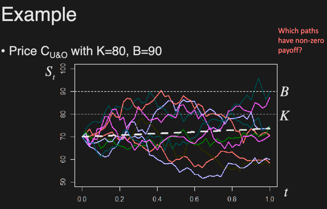
Only the neon purple option has a non-zero payoff, since it hasn’t been knocked out (exceed B), and is above K

Monte Carlo for Barrier Options §

MC for barrier options based on simple discretization leads to biased prices!

All knock-out option prices will be overestimated, because the discretized minima/maxima will not be as extreme as the true ones (there may be some time point we did not simulate, during which the barrier could have been crossed, making the option worthless). Similarly, the knock-in option prices will be underestimated.

Bias can be reduced by increasing number of steps (m) in time discretization, but the computation would become increasingly expensive.

Trade-off between # paths (n) & # steps (m):

• n↑ $⟺$ Var↓ & m↑ $⟺$ Bias↓ (Bias-Variance trade-off)

Reflection principle §

If the path of a Wiener process $W_t$ reaches a value $y$ at time $t$, then the subsequent path after time $s$ has the same distribution as the reflection of the subsequent path about the value $y$.

$$\begin{array}{rl}& P\left(M_t>y,W_t\le x\right)\\ =& P\left(\cancel{M_t>y},\underset{\text{subset of }{M}_t>y}{\underbrace{W_t>y+(y-x)}}\right)\\ =& P\left(W_t>2y-x\right)\end{array}$$

Max of standard BM ~ absolute normal §

For standard BM $\left\{W_t\right\}$, the max by time T, $M_t=\max {\left\{W_t\right\}}_{0\le t\le T}$ is distributed as a folded normal.

We want to find the CDF $P(M_T\le y)$

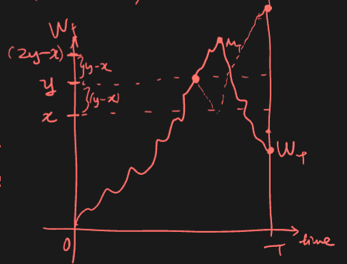
For $x\le y$

$$\begin{array}{rl}P(W_T\le x,M_T\le y)& =P(W_T\le x)-P(W_T\le x,M_T\ge y)\leftarrow P(A\cap B)=P(A)-P(A\cap B^C)\\ & =P(W_T\le x)-P(W_T\ge 2y-x)\leftarrow \text{reflection principle}\end{array}$$

When $x=y$, we have

$$\begin{array}{rl}P(W_T\le y,M_T\le y)& =P(M_T\le y)\\ & =P(W_T\le y)-P(W_T\ge 2y-y)\\ & =P(W_T\le y)-P(W_T\ge y)\\ & =P(W_T\le y)-P(W_T\le -y)\\ & =P(-y\le W_T\le y)\\ & =P(|W_T|\le y)\end{array}$$

Thus $M_T\sim |W_T|$ (consider first line vs last line above).

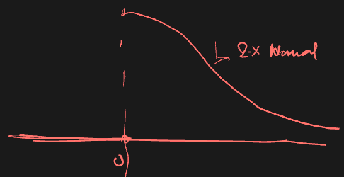
E.g. Find the probability that standard BM $\left\{W_t\right\}$ hits barrier $B=1$ before time $T=1$

Since $W_T\sim N(0,T)$, we have

$$\begin{array}{rl}P(M_1\ge 1)& =P(|W_1|\ge 1)\\ & =2P(Z\ge 1)=2\Phi (-1)=.317862\end{array}$$

Optimal n/m ratio §

MC estimates of $P(\max {\left\{W_t\right\}}_{0\le t\le 1}\ge 1)$ using path discretization w/ different n (paths), m (steps)

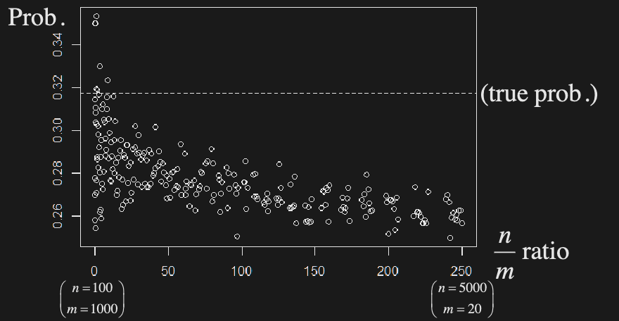
Best MSE lies in the middle:

• High variance when n/m is low
• High bias when n/m is high

E.g. Estimate probability that standard BM hits 1 before time 1, with MC but without bias.

Generate values of $M_T$ directly by generating $W_T$ and setting $M_T=|W_T|$. Then, estimate the probability by the proportion of $M_T^{\prime }s$ that are $>1$

Below are MC estimates of $P(\max {\left\{W_t\right\}}_{0\le t\le 1}\ge 1)$ using direct simulation of $\max \left\{W_t\right\}$ w/ $n=100,000$

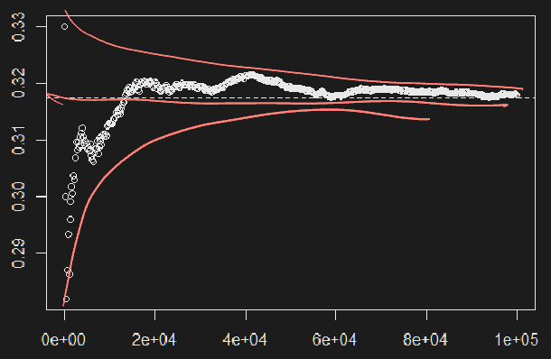
Extrema of Brownian Motion §

• For standard BM $\left\{W_t\right\}$, maximum $M_{\mathrm{T}}$ is distributed as $\left|W_T\right|$
• For arithmetic BM $\left\{X_t\right\}$, the distribution of the maximum is difficult to work with - reflection principle does not work b/c of drift
• However, one can easily simulate random deviates of maximum using Brownian bridge (Brownian motion with fixed end point)
  • Its construction allows for general treatment of extrema of various processes

Consider ABM: $d{X}_t=\mu dt+\sigma d{W}_t$

Conditional on $X_T=b$, the maximum $\left(M_T|X_T\right)={\max }_t\left\{X_t\mid X_T\right\}$ of the Brownian bridge process has a Rayleigh distribution:

$$P\left(M_T\le m\mid X_T=b\right)=1-\exp \left\{-2\frac{m(m-b)}{{\sigma }^{2}T}\right\},\forall m\ge 0\vee b$$

Note that distribution of conditional maximum is independent of the drift, given $X_T=b$

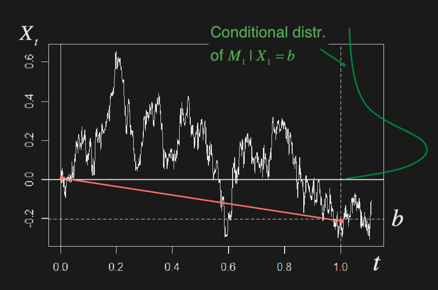
Simulating maxima of ABM §

1. Generate $X_T\sim N\left(\mu T,{\sigma }^{2}T\right)$
2. Generate $U\sim \mathrm{Uniform}(0,1)$
3. Calculate $M_T\mid X_T=\frac{X_T+\sqrt{X_T^2-2{\sigma }^{2}T\log (U)}}{2}$

For maxima of GBM, exponentiate ABM result

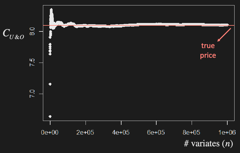
Simulating minima of ABM §

By symmetry, min of ABM with $\mu \equiv$ max of ABM with $-\mu$

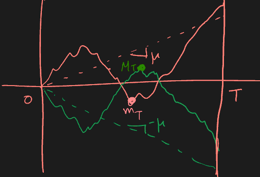
Time Discretization §

Path dependent options generally require simulation of entire discretized path. Exceptions are options depending on maximum (e.g. barrier, look-back).

If prices do not follow GBM, it is generally not possible to simulate from exact distribution of asset prices, so we need to approximate sample path distribution over discrete times

Euler Discretization §

Consider a general SDE where drift/volatility can depend on time $(t)$ and/or process $\left(S_t\right)$

$$d{S}_t=\mu \left(t,S_t\right)dt+\sigma \left(t,S_t\right)d{W}_t$$

There is no general explicit solution for $S_t$, i.e. distribution of $S_t$ is unknown (in closed form)

To approximate the behaviour of $S_t$:

• Discretize time $t_i=i(T/m)=i\Delta t,i=0,\dots ,m$
• Simulate (approx.) path recursively, using $Z_i\stackrel{iid}{\sim }N(0,1),i=1,\dots ,m$

$$S\left(t_i\right)=S\left(t_{i-1}\right)+\mu \left(S\left(t_{i-1}\right),t_{i-1}\right)\Delta t+\sigma \left(S\left(t_{i-1}\right),t_{i-1}\right)\sqrt{\Delta t}{Z}_i$$

To approximate distribution of $S(T)$, generate multiple (#n) discretized paths

W11: Simulation - Variance Reduction Techniques §

Antithetic Variables §

For each normal variate $Z_i$, consider its negative $-Z_i$. Note that they are dependent. For Uniform(0, 1), use $U_i$ and $1-U_i$

Calculate the discounted payoff under both:

$$Y_i=f(Z_i),{\tilde{Y}}_i=f(-Z_i)$$

Estimate price as the mean of the RVs

$${\bar{Y}}_{AV}=\frac{1}{2n}\left(\sum _{i=1}^n{Y}_i+\sum _{i=1}^n{\tilde{Y}}_i\right)=\frac{1}{n}\sum _{i=1}^n\frac{Y_i+{\tilde{Y}}_i}{2}$$

The idea is to balance payoffs of paths with opposite returns.

Pros and cons §

This technique is simple, but not always useful. It only helps if the original and antithetic variates are negatively related.

We can prove this by comparing its variance $V({\bar{Y}}_{AV})$ to the variance of the naive mean $V\left(\frac{1}{2n}{\sum }_{i=1}^{2n}{Y}_i\right)$. Under what condition does the variance get reduced?

Variance reduction proof §

Variance of naive mean:

$$V\left(\frac{1}{2n}\sum _{i=1}^{2n}{Y}_i\right)={\left(\frac{1}{2n}\right)}^2(2nV(Y_i))=\frac{1}{2n}V(Y_i)$$

Variance of antithetic mean:

$$\begin{array}{rl}V({\bar{Y}}_{AV})& =V\left(\frac{1}{2n}\left(\sum _{i=1}^n{Y}_i+\sum _{i=1}^n{\tilde{Y}}_i\right)\right)\\ & ={\left(\frac{1}{2n}\right)}^{2}V\left(\sum _{i=1}^n{Y}_i+\sum _{i=1}^n{\tilde{Y}}_i\right)\\ & ={\left(\frac{1}{2n}\right)}^2\left[nV(Y_i)+nV({\tilde{Y}}_i)+2Cov\left(\sum _{i=1}^n{Y}_i,\sum _{j=1}^n{\tilde{Y}}_j\right)\right]\\ & ={\left(\frac{1}{2n}\right)}^2\left[2nV(Y_i)+2\sum _{i=1}^n\sum _{j=1}^{n}Cov(Y_i,{\tilde{Y}}_j)\right]\\ & ={\left(\frac{1}{2n}\right)}^2\left[2nV(Y_i)+2\sum _{i=1}^{n}Cov(Y_i,{\tilde{Y}}_i)\right]\\ & ={\left(\frac{1}{2n}\right)}^2\left[2nV(Y_i)+2nCov(Y_i,{\tilde{Y}}_i)\right]\\ & =\frac{1}{2n}(V(Y_i)+Cov(Y_i,{\tilde{Y}}_i))\end{array}$$

For $V\left({\bar{Y}}_{AV}\right)<V\left(\frac{1}{2n}{\sum }_{i=1}^{2n}{Y}_i\right)$ to hold, we must have

$$Cov(Y_i,{\tilde{Y}}_i)\le 0$$

Even function => worst case scenario (-Z gives the same value)

Asymptotic distribution of estimator §

Find asymptotic distribution of antithetic variable estimator in terms of moments of $\frac{Y_i+{\tilde{Y}}_i}{2}$

By CLT, we have

$${\bar{Y}}_{AV}\stackrel{approx}{\sim }N\left(E\left(\frac{Y_i+{\tilde{Y}}_i}{2}\right),\frac{1}{n}V\left(\frac{Y_i+{\tilde{Y}}_i}{2}\right)\right)$$

where the mean is

$$\frac{1}{2}(E(Y_i)+E({\tilde{Y}}_i))=\frac{1}{2}2E(Y)=E(Y)=E(f(Z))$$

and the variance is

$$\begin{array}{rl}& \frac{1}{n}\cdot \frac{1}{4}(V(Y_i)+V({\tilde{Y}}_i)+2Cov(Y_i,{\tilde{Y}}_i))\\ =& \frac{1}{4n}(2V(Y_i)+2Cov(Y_i,{\tilde{Y}}_i))\\ =& \frac{1}{2n}(V(Y_i)+Cov(Y_i,\widetilde{Y_i}))\end{array}$$

Example §

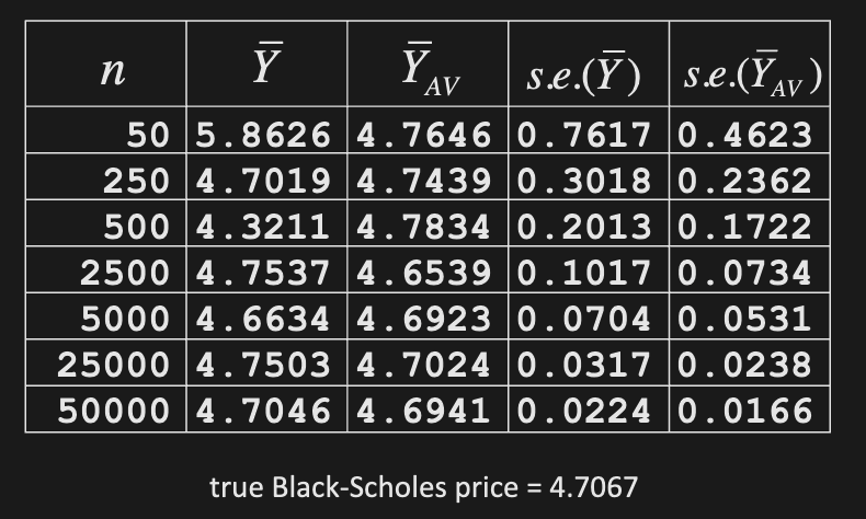
Antithetic variable pricing of a European call

Stratification §

Split the RV domain into equiprobable strata, and draw equal number of variates from within each one

Consider $m$ equiprobable Normal strata $\left\{A_j\right\}$

$$P\left(Z\in A_j\right)=\frac{1}{m}\text{ for }j=1,\dots ,m,\text{and }Z\sim N(0,1)$$

Stratified estimator of $Y=f(Z)$ is given by

$$\begin{array}{rl}{\bar{Y}}_{Str}& =\frac{1}{m}\sum _{j=1}^m{\bar{Y}}^{(j)}\\ & =\frac{1}{m}\sum _{j=1}^m\left(\frac{1}{n}\sum _{i=1}^{n}f\left(Z_i^{(j)}\right)\right)\end{array}$$

where ${\bar{Y}}^{(j)}$ is the estimator within each stratum $j$, and $Z_i^{(j)}\stackrel{iid}{\sim }N\left(0,1\mid Z_i^{(j)}\in A_j\right),j=1,\dots ,m$

Mean of estimator §

Verify that ${\bar{Y}}_{Str}$ is an unbiased estimator of $E(f(Z))$

$$\begin{array}{rl}E({\bar{Y}}_{Str})& =E\left(\frac{1}{m}\sum _{j=1}^m{\bar{Y}}^{(j)}\right)\\ & =\frac{1}{m}\sum _{j=1}^{m}E({\bar{Y}}^{(j)})\\ & =\frac{1}{m}\sum _{j=1}^{m}E\left(\frac{1}{n}\sum _{i=1}^n{Y}_j^{(j)}\right)\\ & =\frac{1}{m}\sum _{j=1}^m\frac{1}{n}\sum _{i=1}^n\underset{E(Y|Z\in A_j)}{\underbrace{E(Y_i^{(j)})}}\\ & =\underset{P(Z\in A_j)}{\underbrace{\frac{1}{m}}}\sum _{j=1}^m\frac{1}{n}nE(f(Z)|Z\in A_j)\\ & =\sum _{j=1}^{m}E(f(Z)|Z\in A_j)P(Z\in A_j)\\ & =E(f(Z))\text{by LOTP}\\ & =E(Y)\end{array}$$

Variance reduction proof §

Show that $V[{\bar{Y}}_{Str}]<V[\bar{Y}]\text{, where }\bar{Y}=\frac{1}{nm}{\sum }_{i=1}^{nm}f\left(Z_i\right)$

$$\begin{array}{rl}V(\bar{Y})& =V\left(\frac{1}{nm}\sum _{i=1}^{nm}{Y}_i\right)=\frac{1}{nm}V(Y_i)=\frac{1}{nm}\left(E(Y_i^2)-(E(Y_i){)}^2)\right)=\frac{1}{nm}(E(f^2(Z))-{\mu }^2)\\ V({\bar{Y}}_{Str})& =V\left(\frac{1}{m}\sum _{j=1}^m{\bar{Y}}^{(j)}\right)=\frac{1}{m^2}\sum _{j=1}^{m}V({\bar{Y}}^{(j)})=\frac{1}{m^2}\sum _{j=1}^{m}V\left(\frac{1}{n}\sum _{i=1}^n{Y}_i^{(j)}\right)=\frac{1}{m^2{n}^2}\sum _{j=1}^m\sum _{i=1}^{n}V(Y_i^{(j)})\\ & =\frac{1}{m^2{n}^2}\sum _{j=1}^{m}nV(Y^{(j)})=\frac{1}{m^{2}n}\sum _{j=1}^{m}V(Y|Z\in A_j)=\frac{1}{m^{2}n}\sum _{j=1}^m(E(f^2(Z)|Z\in A_j)-(E(f(Z))|Z\in A_j{)}^2)\\ & =\frac{1}{mn}\left\{\underset{E(f^2(Z))}{\underbrace{\sum _{j=1}^{m}E(f^2(Z)|Z\in A_j)\underset{P(Z\in A_j)}{\underbrace{\frac{1}{m}}}}}-\frac{1}{m}\sum _{j=1}^m(\underset{{\mu }_j}{\underbrace{E(f(Z)|Z\in A_j)}}{)}^2\right\}\\ & =\frac{1}{mn}\left\{E(f^2(Z))-\frac{1}{m}\sum _{j=1}^m{\mu }_j^2\right\}\end{array}$$

So we have $V[{\bar{Y}}_{Str}]<V[\bar{Y}]$ since $\frac{1}{m}{\sum }_{j=1}^m{\mu }_j^2\ge {\mu }^2$ by Jensen’s inequality

So for $f(x)=x^2$, a convex function, we have

$$\underset{=\frac{1}{m}{\sum }_{j=1}^m{\mu }_j^2}{\underbrace{E(x^2)}}\ge \underset{={\mu }^2={\left(\frac{1}{m}{\sum }_{j=1}^m{\mu }_j\right)}^2}{\underbrace{(E(x){)}^2}}$$

Pros and cons §

This method ensures equal representation of each stratum in the RV’s domain. It always reduces variance.

It works best when target RV (payoff) changes over its domain, i.e. is highly variable (as opposed to a flat payoff).

It is computationally difficult for multidimensional RV’s. Getting the conditional distribution within each stratum can be difficult, and the CDF is often unknown.

Example §

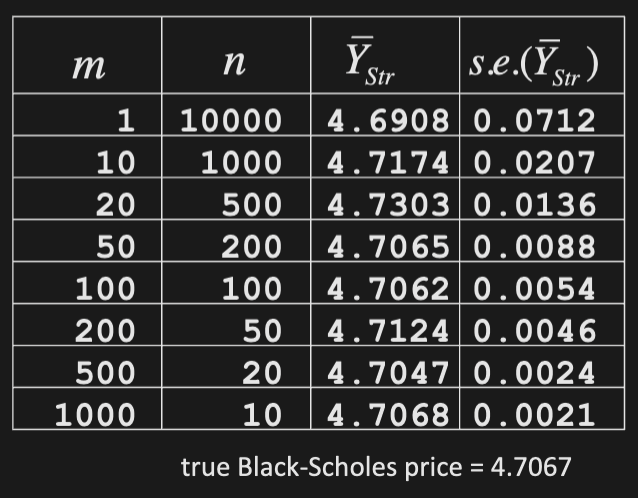
Stratified pricing of a European call

Control Variates §

Estimate $E[Y]=E[f(Z)]$ using MC: generate iid $Z_i$ and use

$$\bar{Y}=\sum _{i=1}^n{Y}_i/n=\sum _{i=1}^{n}f\left(Z_i\right)/n$$

where $f(\cdot )$ is option’s discounted payoff

Assume there is another option with payoff $g(\cdot )$ whose price $E[X]=E[g(Z)]$ is known. The idea is to use MC with the same variates to estimate both $E[Y]$ and $E[X]$, but adjust the estimate $\bar{Y}$ to take into account the error of estimate $\bar{X}$. E.g. if $\bar{X}$ underestimates $E[X]$, then increase $\bar{Y}$.

Adjust $\bar{Y}$ for estimation error $\bar{X}-E[X]$ linearly, as

$$\bar{Y}(b)=\bar{Y}-b(\bar{X}-E[X])$$

where the coefficient $b$ controls adjustment.

Mean of estimator (unbiased proof) §

Show that $\bar{Y}(b)$ is unbiased for any $b$ (provided $\bar{Y},\bar{X}$ are unbiased)

$$\begin{array}{rl}E(\bar{Y}(b))& =E(\bar{Y}-b(\bar{X}-E(X)))\\ & =E(\bar{Y})-b(E(\bar{X})-E(X))\\ & =E(Y)-b(\underset{\text{0 adjustment}}{\underbrace{E(X)-E(X)}})\\ & =E(Y)\end{array}$$

Variance of estimator §

$$\begin{array}{rl}\mathbb{V}[\bar{Y}(b)]& =\mathbb{V}[\bar{Y}-b(\bar{X}-\mathbb{E}(X))]=\mathbb{V}[\bar{Y}-b\bar{X}]\\ & =\mathbb{V}(\bar{Y})+b^2\mathbb{V}(\bar{X})-2b\mathrm{Cov}(\bar{Y},\bar{X})\\ & =\frac{1}{n}\mathbb{V}(Y)+b^2\frac{1}{n}\mathbb{V}(X)-2b\mathrm{Cov}(\frac{1}{n}\sum _{i=1}^n\underset{Y_i}{\underbrace{f\left(X_i\right)}},\frac{1}{n}\sum _{i=1}^n\underset{X_i}{\underbrace{g\left(Z_i\right)}})\\ & =\frac{1}{n}\mathbb{V}(Y)+b^2\frac{1}{n}\mathbb{V}(X)-2b\frac{1}{n^2}n\mathrm{Cov}(f(Z)),g(Z))\\ & =\frac{1}{n}\left[{\sigma }_Y^2+b^2{\sigma }_X^2-2b{\sigma }_{XY}\right]\end{array}$$

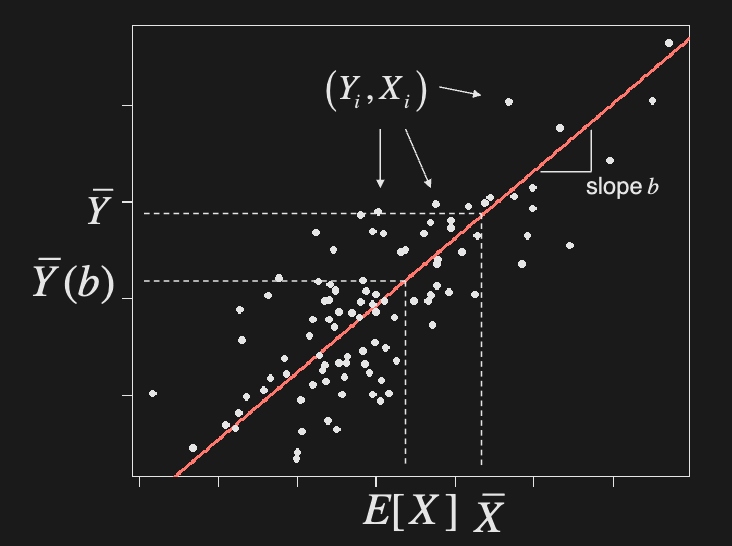
Optimal value of adjustment coefficient §

Show that the optimal value of $b$ is $b^{\ast }=\frac{Cov(X,Y)}{Var(X)}$. This is the regression slope coefficient.

$$\begin{array}{rl}\frac{\partial }{\partial b}\mathbb{V}(\bar{Y}(b))& =0\\ \frac{\partial }{\partial b}\left(\frac{1}{n}\left[{\sigma }_Y^2+b^2{\sigma }_X^2-2b{\sigma }_{xXY}\right]\right)& =0\\ b{\sigma }_X^2-{\sigma }_{XY}& =0\\ b& =\frac{{\sigma }_{XY}}{{\sigma }_X^2}=\frac{{\rho }_{XY}{\sigma }_X{\sigma }_Y}{{\sigma }_X^2}={\rho }_{XY}\frac{{\sigma }_Y}{{\sigma }_X}\end{array}$$

In practice, $\mathrm{Cov}[X,Y],\mathrm{Var}[X]$ are unknown, so we estimate $b^{\ast }$ using MC sample

$$\hat{b}=\frac{{\sum }_{i=1}^n\left(X_i-\bar{X}\right)\left(Y_i-\bar{Y}\right)}{{\sum }_{i=1}^n{\left(X_i-\bar{X}\right)}^2}$$

Optimal variance §

Show that the optimal variance is $V(\bar{Y}(b^{\ast }))=V(\bar{Y})(1-{\rho }_{XY}^2)$

$$\begin{array}{rl}\mathbb{V}\left[\bar{Y}\left(b^{\ast }\right)\right]& =\frac{1}{n}\left({\sigma }_Y^2-(b^{\ast }{)}^2{\sigma }_X^2-2b^{\ast }{\sigma }_{XY}\right)\\ & =\frac{1}{n}\left({\sigma }_Y^2+{\left({\rho }_{XY}\frac{{\sigma }_Y}{{\sigma }_X}\right)}^2{\sigma }_X^2-2\left({\rho }_{XY}\frac{{\sigma }_Y}{{\sigma }_X}\right){\sigma }_X{\sigma }_Y{\rho }_{XY}\right)\\ & =\frac{1}{n}\left({\sigma }_Y^2+{\rho }_{XY}^2{\sigma }_Y^2-2{\rho }_{XY}^2{\sigma }_Y^2\right)\\ & =\frac{1}{n}{\sigma }_Y^2\left(1-{\rho }_{XY}^2\right)\\ & =\mathbb{V}(\bar{Y})\left(1-{\rho }_{XY}^2\right)\end{array}$$

In practice, we need to use sample estimates of $\mathrm{Var}[\bar{Y}],{\rho }_{XY}$

Correlation of control §

Good control variates have high absolute correlation with option payoff (high ${\rho }_{XY}$)

• In-the-money call: ${\rho }_{XY}\approx 1$
  • $Cov(S_T,S_T-K)>0$
• Out-of-the-money call: ${\rho }_{XY}\approx 0$
  • $Cov(S_T,0)=0$
• In-the-money put: ${\rho }_{XY}\approx -1$
• Out-of-the-money put: ${\rho }_{XY}\approx 0$

Example §

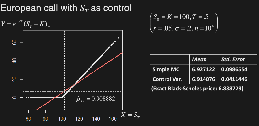
Price European option using final asset price ($S_t$) as control, assuming GBM with $r,\sigma$

• $X=S_T=g(Z)=S_0\exp \left\{\left(r-\frac{{\sigma }^2}{2}\right)T+\sigma \sqrt{T}Z\right\}$
• $E[X]=E\left[S_T\right]=S_0{e}^{rT}$

Importance Sampling §

We can reduce variance by changing the distribution (probability measure) from which paths are generated to give more weight to important outcomes, thereby increasing sample efficiency. The performance of this method relies heavily on the equivalent measure being used.

E.g. for European call, we put more weight to paths with positive payoff (i.e. paths for which we exercise)

Let $\varphi (z)$ be pdf of $Z$, we want to estimate

$$\alpha =E_{\varphi }[f(Z)]={\int }_{z}f(z)\varphi (z)dz$$

Using simple MC, generate sample $Z_i{\sim }^{iid}\varphi ,i=1,\dots ,n$. The estimate is thus $\hat{\alpha }={\sum }_{i=1}^{n}f\left(Z_i\right)/n$ If we have sample $Z_i^{\prime }\stackrel{iid}{\sim }\psi ,i=1,\dots ,n$ from a new pdf $\psi$, we can still estimate $\alpha$ as follows

$$\begin{array}{rl}\alpha ={\int }_{z}f(z)\varphi (z)dz& =\underset{\int x{f}_X(x)dx=E(X)}{\underbrace{{\int }_{z}f(z)\frac{\varphi (z)}{\psi (z)}\psi (z)dz=E_{\psi }\left[f\left(Z^{\prime }\right)\frac{\varphi \left(Z^{\prime }\right)}{\psi \left(Z^{\prime }\right)}\right]}}\\ & \Rightarrow {\hat{\alpha }}^{\prime }=\frac{1}{n}\sum _{i=1}^{n}f\left(Z_i^{\prime }\right)\frac{\varphi \left(Z_i^{\prime }\right)}{\psi \left(Z_i^{\prime }\right)}\end{array}$$

Mean of estimator §

$$\begin{array}{rl}{E}_{\psi }[{\hat{\alpha }}^{\prime }]& =E_{\psi }\left(\frac{1}{n}\sum _{i=1}^{n}f(Z_i^{\prime })\frac{\varphi (Z_i^{\prime })}{\psi (Z_i^{\prime })}\right)\\ & =\frac{1}{n}\sum _{i=1}^n{E}_{\psi }\left[f(Z^{\prime })\frac{\varphi (Z^{\prime })}{\psi (Z^{\prime })}\right]\\ & ={\int }_{-\infty }^{\infty }\underset{value}{\underbrace{f(Z^{\prime })\frac{\varphi (Z^{\prime })}{\psi (Z^{\prime })}}}\underset{prob}{\underbrace{\psi (Z^{\prime })}}d{Z}^{\prime }\\ & ={\int }_{-\infty }^{\infty }f(Z^{\prime })\varphi (Z^{\prime })d{Z}^{\prime }\\ & =E_{\varphi }[f(Z)]\\ & =\alpha \end{array}$$

Note that this estimate is unbiased (provided simple MC estimate $\hat{\alpha }$ is unbiased).

Variance of estimator §

$$\begin{array}{rl}{V}_{\psi }({\hat{\alpha }}^{\prime })& =V_{\psi }\left(\frac{1}{n}\sum _{i=1}^{n}f(Z_i^{\prime })\frac{\varphi (Z_i^{\prime })}{\psi (Z_i^{\prime })}\right)\\ & =\frac{1}{n}{V}_{\psi }\left(f(Z_i^{\prime })\frac{\varphi (Z_i^{\prime })}{\psi (Z_i^{\prime })}\right)\\ & =\frac{1}{n}\left\{{\mathbb{E}}_{\psi }\left[{\left(f(z^{\prime })\frac{\varphi (z^{\prime })}{\psi (z^{\prime })}\right)}^2\right]-{\left({\mathbb{E}}_{\psi }\left[f(z^{\prime })\frac{\varphi (z^{\prime })}{\psi (z^{\prime })}\right]\right)}^2\right\}\end{array}$$

Variance reduction proof & condition §

Show that ${\mathrm{Var}}_{\psi }\left[{\hat{\alpha }}^{\prime }\right]\le {\mathrm{Var}}_{\varphi }[\hat{\alpha }]⟺E_{\varphi }\left[f^2(Z)\frac{\varphi (Z)}{\psi (Z)}\right]\le E_{\varphi }\left[f^2(Z)\right]$

$$\begin{array}{rl}{\mathbb{V}}_{\psi }\left[{\hat{\alpha }}^{\prime }\right]& \le {\mathbb{V}}_{\varphi }[\hat{\alpha }]\\ \frac{1}{n}\left\{{\mathbb{E}}_{\psi }\left[{\left(f(z^{\prime })\frac{\varphi (z^{\prime })}{\psi (z^{\prime })}\right)}^2\right]-{\alpha }^2\right\}& \le \frac{1}{n}\left\{{\mathbb{E}}_{\varphi }\left[f^2(z)\right]-{\alpha }^2\right\}\\ {\mathbb{E}}_{\psi }\left[f^2(z^{\prime })\frac{{\varphi }^2(z^{\prime })}{{\psi }^2(z^{\prime })}\right]& \le {\mathbb{E}}_{\varphi }\left[f^2(z)\right]\end{array}$$

The LHS is equivalent to

$$\begin{array}{rl}\int \underbrace{f^2(z^{\prime })\frac{{\varphi }^2(z^{\prime })}{{\psi }^2(z^{\prime })}}\psi (z^{\prime })d{z}^{\prime }& =\int f^2(z^{\prime })\underbrace{\frac{\varphi (z^{\prime })}{\psi (z^{\prime })}\varphi (z^{\prime })}d{z}^{\prime }\\ & ={\mathbb{E}}_{\varphi }\left[f^2(z)\frac{\varphi (z)}{\psi (z)}\right]\end{array}$$

Optimal variance condition §

Show that for positive $f$, $Va{r}_{\psi }[{\hat{\alpha }}^{\prime }]=0$ if $\psi (z)\propto f(z)\varphi (z)$

i.e. importance sampling works best when new pdf $\psi$ resembles $f\times \varphi$ (payoff $\times$ original pdf)

$$\begin{array}{rl}\psi (z)& =\frac{1}{c}f(z)\varphi (z)\\ \int \psi (z)dz& =\int \frac{1}{c}f(z)\varphi (z)dz=1\\ c& =\int f(z)\varphi (z)dz\\ & =E_{\varphi }(f(z))=\alpha \end{array}$$

$$\begin{array}{rl}{\mathbb{V}}_{\psi }\left[{\hat{\alpha }}^{\prime }\right]& =\frac{1}{n}\left\{{\mathbb{E}}_{\psi }\left[{\left(f\left(z^{\prime }\right)\frac{\varphi \left(z^{\prime }\right)}{\psi \left(z^{\prime }\right)}\right)}^2\right]-{\alpha }^2\right\}\\ & =\frac{1}{n}\left\{{\mathbb{E}}_{\psi }\left[{\left(\frac{f\left(z^{\prime }\right)\varphi \left(z^{\prime }\right)}{\frac{1}{c}f\left(z^{\prime }\right)\varphi \left(z^{\prime }\right)}\right)}^2\right]-{\alpha }^2\right\}\\ & =\frac{1}{n}\{\underset{{\alpha }^2}{\underbrace{{\mathbb{E}}_{\psi }\left[c^2\right]}}-{\alpha }^2\}\\ & =\frac{1}{n}\left({\alpha }^2-{\alpha }^2\right)=0\end{array}$$

Multiple random variates §

Importance sampling can be extended to multiple random variates per path

For example, for a path-dependent option with payoff $f\left(Z_1,\dots ,Z_m\right)$, which is a function of m variates forming discretized path, the mean of the estimate is

$$E_{\varphi }\left[f\left(Z_1,\dots ,Z_m\right)\right]=E_{\psi }\left[f\left(Z_1^{\prime },\dots ,Z_m^{\prime }\right)\frac{\varphi \left(Z_1^{\prime },\dots ,Z_m^{\prime }\right)}{\psi \left(Z_1^{\prime },\dots ,Z_m^{\prime }\right)}\right]$$

If in addition, $Z_j\stackrel{iid}{\sim }{\varphi }_j$, $Z_j^{\prime }\stackrel{iid}{\sim }{\psi }_j$, then

$$E_{\varphi }\left[f\left(Z_1,\dots ,Z_m\right)\right]=E_{\psi }\left[f\left(Z_1^{\prime },\dots ,Z_m^{\prime }\right)\prod _{j=1}^m\frac{{\varphi }_j\left(Z_j^{\prime }\right)}{{\psi }_j\left(Z_j^{\prime }\right)}\right]$$

Example §

Consider a deep out-of-the-money European call with $S_0=50,K=65$

With simple MC, generate final prices as

$$S_T=S_0{e}^Z,\text{ where }Z\sim \varphi =N\left(\left(r-\frac{{\sigma }^2}{2}\right)T,{\sigma }^{2}T\right)$$

Which of the following is a better candidate for $\psi$ ?

$$Z^{\prime }\sim \psi =N\left(\log \left(\frac{90}{50}\right)-\frac{{\sigma }^2}{2}T,{\sigma }^{2}T\right)\text{ or }N\left(\log \left(\frac{30}{50}\right)-\frac{{\sigma }^2}{2}T,{\sigma }^{2}T\right)$$

The former, since it is ITM. We want to simulate from distributions with higher means (closer to $K=65$).

W12: Optimization in Finance §

Most real world problems involve making decisions, often under uncertainty. Making good/optimal decisions typically involves some optimization.

In finance, we must typically decide how to invest over time and across assets.

E.g. mean-variance analysis or Kelly criterion

Types of Optimization Problems §

• Straightforward (closed form or polynomial complexity):
  • Linear, quadratic, convex
  • Equality/linear/convex constraints
• Difficult:
  • Discrete optimization (discrete variable)
    • E.g. indivisible assets, transaction costs
  • Dynamic optimization (previous decisions affect future ones)
    • Investing overtime
  • Stochastic optimization (uncertainty)

Discrete & Dynamic Optimization §

Assume you can perfectly foresee the price of a stock. You want to make optimal use of such knowledge, assuming

• you can only trade integer units of the asset
• every transaction costs you a fixed amount
• you cannot short sell the asset

This is a discrete, dynamic optimization problem. Although there is no randomness (we have perfect knowledge), the problem is not trivial.

We could consider all possible strategies, but that would be expensive - the search space size is $2^n$.

We can use dynamic programming (backward induction) instead:

• At any time t, there are 2 states: owning or not owning the asset
• The optimal value of each state at t = the best option out of transitioning to another state + the optimal value of that state at t+1
• Start from the end, and consider optimal value going backwards to discover the best strategy

E.g. Find evolution of value, assuming no position at $t=0$ and $t>n$

Let $S(t)=$ asset price at $t$, $tc=$ transaction cost, $V_{np}(t)=$ opt. value for no position at $t$, $V_{lp}(t)=$ opt. value for long position at $t$

state \ time	t=1	t=2	t=3=n	> n
no position	$V_{np}(1)=\max \{0+V_{np}(2),-S(1)-tc+V_{lp}(2)\}$	$V_{np}(2)=\max \{0+V_{np}(3),-S(2)-tc+V_{lp}(3)\}$	$V_{np}(3)=0$	0
long position	/	$V_{lp}(2)=\max \{0+V_{lp}(3),S(2)-tc+V_{np}(3)\}$	$V_{lp}(3)=S(3)-tc$	/

E.g.

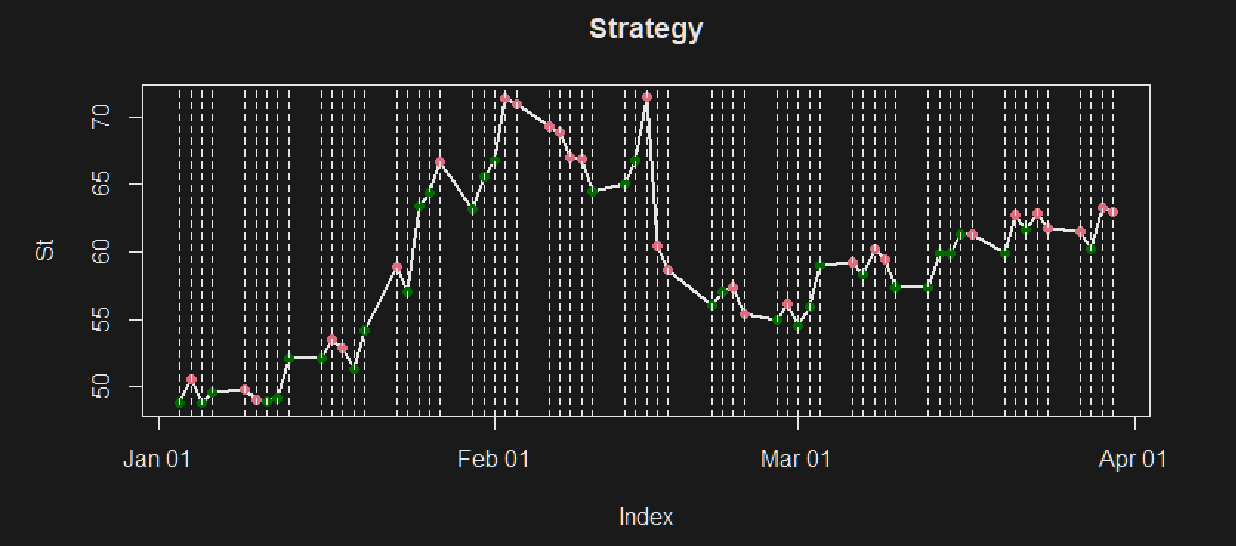
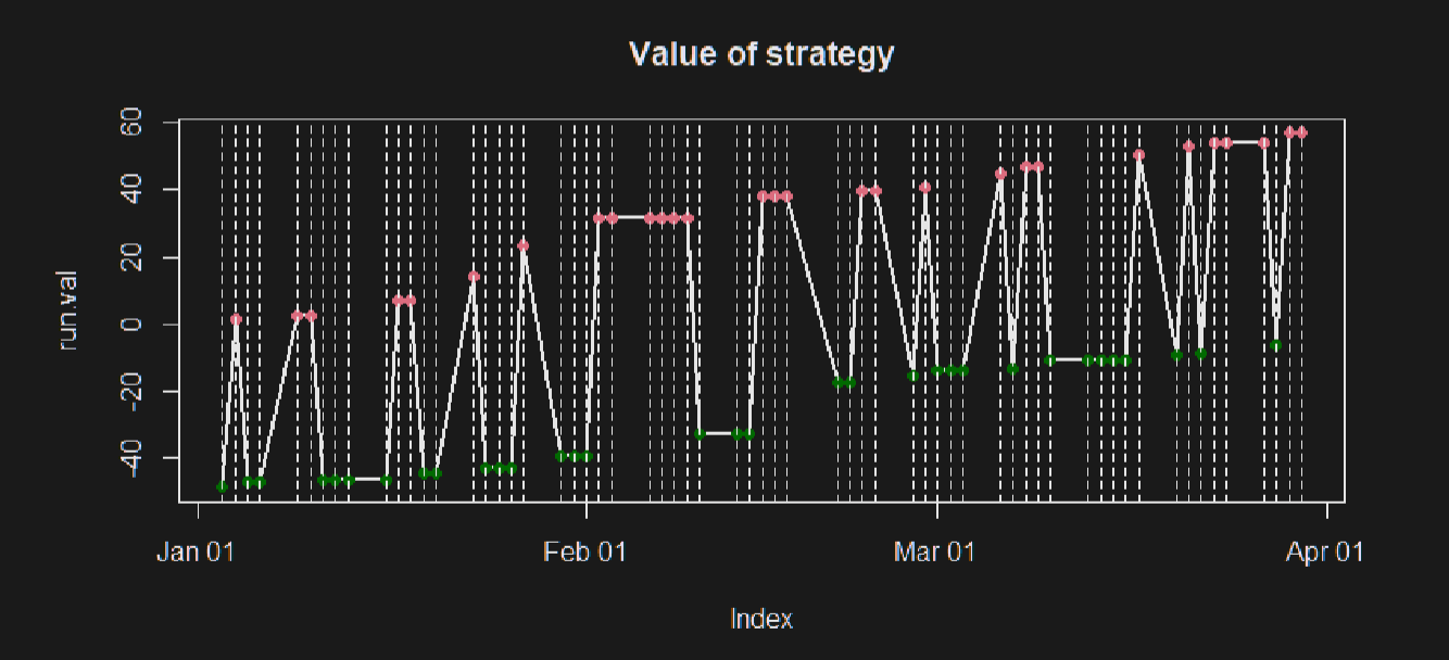
Stochastic Optimization §

Consider a similar problem without exact price knowledge (e.g. prices follow binomial tree with some probabilities)

We want to find the best trading strategy (which maxes the expected P&L)

Define the following:

• $X_t$ is the state RV (price and position, e.g. long/short)
• $a_t$ is action (change in state e.g. buy/sell)
• $f_t$ is a reward function (e.g. cashflow)

We want to maximize expected reward over stochastic actions

Letting $V(t,X_t)$ be the optimal value function, we have

$$\begin{array}{rl}V\left(t,X_t\right)& =\underset{a_{t\to T}}{\max }\left\{\mathbb{E}\left[\sum _{s=t}^{T}f\left(s,X_s,a_s\right)\mid X_t\right]\right\}\\ & =\underset{a_{t\to T}}{\max }\left\{f\left(t,X_t,a_t\right)+\mathbb{E}\left[\sum _{s=t+1}^{T}f\left(s,X_s,a_s\right)\mid X_t\right]\right\}\\ & =\underset{a_t}{\max }\left\{f\left(t,X_t,a_t\right)+\underset{a_{(t+1)\to T}}{\max }\left\{\mathbb{E}\left[\sum _{s=t+1}^{T}f\left(s,X_s,a_s\right)\mid X_t\right]\right\}\right\}\\ & =\underset{a_t}{\max }\left\{f\left(t,X_t,a_t\right)+\mathbb{E}\left[\underset{a_{(t+1)\to T}}{\max }\left\{\mathbb{E}\left[\sum _{s=t+1}^{T}f\left(s,X_s,a_s\right)\mid X_{t+1}^{\left(a_t\right)}\right]\right\}\mid X_t\right]\right\}\\ & =\underset{a_t}{\max }\left\{f\left(t,X_t,a_t\right)+\mathbb{E}\left[V\left(t+1,X_{t+1}^{\left(a_t\right)}\right)\mid X_t\right]\right\}\end{array}$$

E.g. Consider the following Binomial tree, with up/down probability of 1/2:

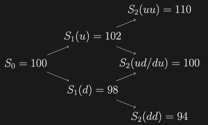
Find the optimal strategy that maximizes the expected $\mathrm{P}/\mathrm{L}$ assuming you can long and short the asset, and there is a transaction cost of $0.1/share. Note that there are three possible states now (long, neutral, short), and $3^3=27$ possible strategies. Find the optimal strategy and its value using dynamic programming, and optionally verify it with an exhaustive search.

Solution: It is not difficult to reason that the best strategy is to go long at $u$ and short at $d$, since the up paths have positive expected $\mathrm{P}/\mathrm{L}$ and the down paths have negative expected $\mathrm{P}/\mathrm{L}$ (greater than the transaction costs), and this strategy minimizes the expected costs (you only long/short when you need). You can actually verify this by calculating the expected $\mathrm{P}/\mathrm{L}$ of all 27 strategies by brute force (e.g., in R) to get:

Strategy	Expected P//L
s,s,s	-1-2tc
s,s,n	-1.5-2tc
s,s,l	-2-3tc
s,n,s	0.5-2tc
s,n,n	0-2tc
s,n,l	-0.5-3tc
s,l,s	2-3tc
s,l,n	1.5-3tc
s,l,l	1-4tc
n,s,s	-1-2tc
n,s,n	-1.5-1tc
n,s,l	-2-2tc
n,n,s	0.5-1tc
n,n,n	0
n,n,l	-0.5-1tc
n,l,s	2-2tc
n,l,n	1.5-1tc
n,l,l	1-2tc
l,s,s	-1-4tc
l,s,n	-1.5-3tc
l,s,l	-2-3tc
l,n,s	0.5-3tc
l,n,n	0-2tc
l,n,l	-0.5-2tc
l,l,s	2-3tc
l,l,n	1.5-2tc
l,l,l	1-2tc

But you can drastically reduce the required calculations using backward induction/dynamic programming. Let $V\left(t,\left(S_t,p\right)\right)$ denote the optimal value at time $t$ for price $S_t$ and “position” $p\in \{s,n,l\}$.

At time $t=2$ we have:

$$\begin{array}{rl}V(2,(110,l))& =110-tc\\ V(2,(110,n))& =0\\ V(2,(110,s))& =-110-tc\\ & \\ V(2,(100,l))& =100-tc\\ V(2,(100,n))& =0\\ V(2,(100,s))& =-100-tc\\ & \\ V(2,(94,l))& =94-tc\\ V(2,(94,n))& =0\\ V(2,(94,s))& =-94-tc\end{array}$$

At time $t=1$ and $S_1=102$, we have

$$\begin{array}{rl}V(1,(102,l))& =\max \left\{\begin{array}{l}0+\frac{1}{2}[V(2,(110,l))+V(2,(100,l))]=105-tc,\\ 102-tc+\frac{1}{2}[V(2,(110,n))+V(2,(100,n))]=102-tc,\\ 2(102-tc)+\frac{1}{2}[V(2,(110,s))+V(2,(100,s))]=99-3tc\end{array}\right\}\\ & =105-tc\\ V(1,(102,n))& =\max \left\{\begin{array}{l}-102-tc+\frac{1}{2}[V(2,(110,l))+V(2,(100,l))]=3-2tc,\\ 0+\frac{1}{2}[V(2,(110,n))+V(2,(100,n))]=0\\ 102-tc+\frac{1}{2}[V(2,(110,s))+V(2,(100,s))]=-3-2tc\end{array}\right\}\\ & =3-2tc\\ V(1,(102,s))& =\max \left\{\begin{array}{l}-2(102+tc)+\frac{1}{2}[V(2,(110,l))+V(2,(100,l))]=-99-3tc,\\ -102-tc+\frac{1}{2}[V(2,(110,n))+V(2,(100,n))]=-102-tc,\\ 0+\frac{1}{2}[V(2,(110,s))+V(2,(100,s))]=-105-tc\end{array}\right\}\\ & =-99-3tc\\ & \end{array}$$

At time $t=1$ and $S_1=98$, we have

$$\begin{array}{rl}V(1,(98,l))& =\max \left\{\begin{array}{l}0+\frac{1}{2}[V(2,(100,l))+V(2,(94,l))]=97-tc\\ 98-tc+\frac{1}{2}[V(2,(100,n))+V(2,(94,n))]=98-tc\\ 2(98-tc)+\frac{1}{2}[V(2,(100,s))+V(2,(94,s))]=99-3tc\end{array}\right\}\\ & =99-3tc\\ V(1,(98,n))& =\max \left\{\begin{array}{l}-98-tc+\frac{1}{2}[V(2,(100,l))+V(2,(94,l))]=-1-2tc,\\ 0+\frac{1}{2}[V(2,(100,n))+V(2,(94,n))]=0\\ 98-tc+\frac{1}{2}[V(2,(100,s))+V(2,(94,s))]=1-2tc\end{array}\right\}\\ & =1-2tc\\ V(1,(98,s))& =\max \left\{\begin{array}{l}-2(98+tc)+\frac{1}{2}[V(2,(100,l))+V(2,(94,l))]=-99-3tc,\\ -98-tc+\frac{1}{2}[V(2,(100,n))+V(2,(94,n))]=-98-tc,\\ 0+\frac{1}{2}[V(2,(100,s))+V(2,(94,s))]=-97-tc\end{array}\right\}\\ & =-97-tc\\ & \end{array}$$

At time $t=0$ and state $\mathrm{n}$ (the only relevant one at the start) we have

$$\begin{array}{rl}V(0,(100,n))& =\max \left\{\begin{array}{l}-100-tc+\frac{1}{2}[V(1,(102,l))+V(1,(98,l))]\\ 0+\frac{1}{2}[V(1,(102,n))+V(1,(98,n))]\\ +100-tc+\frac{1}{2}[V(1,(102,s))+V(1,(98,s))]\end{array}\right\}\\ & =\max \left\{\begin{array}{l}-100-tc+\frac{1}{2}[(105-tc)+(99-3tc)]=2-3tc,\\ 0+\frac{1}{2}[(3-2tc)+(1-2tc)]=2-2tc,\\ +100-tc+\frac{1}{2}[(-99-3tc)+(-97-tc)]=2-3tc\end{array}\right\}\\ & =2-2tc\end{array}$$